Originally a guest post 11 December 2018 at Climate Etc
An observational estimate of transient (multidecadal) warming relative to cumulative CO2 emissions is little over half that per IPCC AR5 projections.
AR5 claims that CO2-caused warming would be undiminished for 1000 years after emissions cease, but observations indicate that it would halve.
Introduction
In recent years climate scientists and policymakers have increasingly focused on the sensitivity of the climate system to cumulative carbon emissions, which provides a simple link between politically-chosen maximum global warming targets and implicit carbon emission budgets. Figure 1 below, a reproduction of IPCC AR5 Figure SPM.10, shows how warming projected by climate models progresses during the four AR5 emission scenarios, RCP2.6 to RCP8.5. This chart appears to be of key importance so far as policymaking is concerned.
The multimodel mean warming response to cumulative carbon emissions in Figure 1 is almost identical for all scenarios, and is approximately linear. These are only model projections, and there are wide differences between the responses of the various models (shown by the coloured plume). However, there are reasons to believe that there is a fundamental link between cumulative carbon emissions and warming, at least in equilibrium. In this article I shall attempt to quantify this relationship, using observationally-based estimates rather than complex climate-carbon cycle models. The results suggest that the AR5 projections are over pessimistic by a factor of almost two in this century, and by even more in the long run.
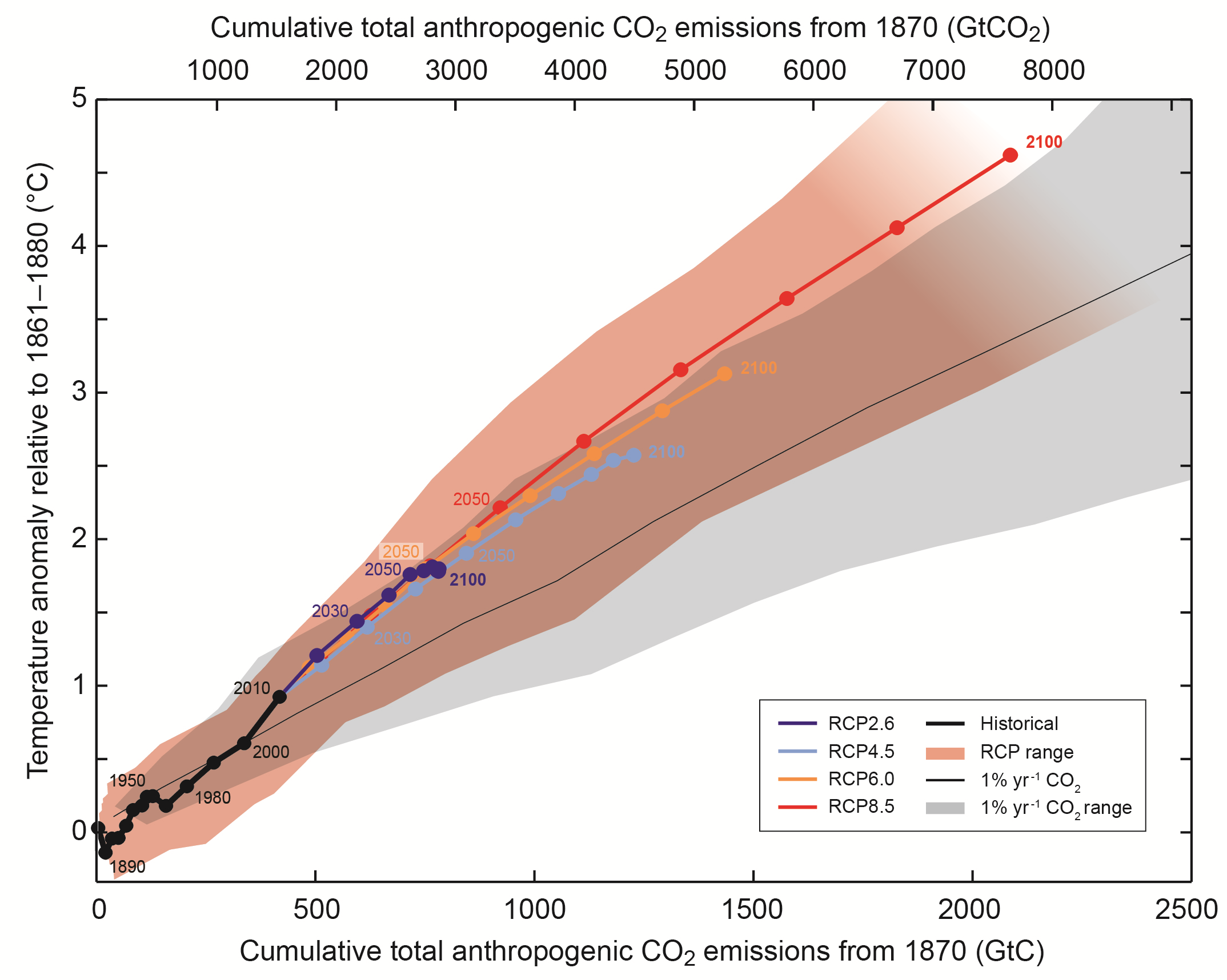
Figure 1. Reproduction of IPCC AR5 WG1 Figure SPM.10: Simulated global mean surface temperature increase as a function of cumulative total global CO2 emissions from various lines of evidence. Multi-model results from a hierarchy of climate-carbon cycle models for each RCP until 2100 are shown with coloured lines and decadal means (dots). The multi-model mean and range simulated by CMIP5 models, forced by a CO2 increase of 1% per year, is given by the thin black line and grey area. The 1% per year CO2 simulations exhibit lower warming than those driven by RCPs, which include additional non-CO2 forcings. Temperature values are given relative to the 1861−1880 base period, emissions are post 1870.[i]
There are two principal metrics for sensitivity to cumulative carbon emissions. The best known is the transient response to carbon emissions (TCRE).[ii] This measures the change in global mean surface temperature (GMST) at the end of a period, typically of the order of a century long, during which CO2 is emitted smoothly. TCRE is stated per 1000 GtC (≡ 1 TtC) emissions, and usually assumes a total of 1000 GtC is emitted. Note that 1000 GtC is the carbon content of 3667 GtCO2.
In CMIP5 earth system models (ESMs), which couple carbon cycle models with atmosphere-ocean global climate models, TCRE ranges from 0.8°C to 2.4°C, with a mean of 1.6°C.[iii] The assessment in AR5, which largely mirrors the CMIP5 ESM range, was that the TCRE is likely between 0.8°C to 2.5°C, for cumulative CO2 emissions less than about 2000 GtC, until the time at which temperatures peak. The multi-model mean TCRE under the middling RCP4.5 and RCP6.0 scenarios shown in Figure SPM.10 is 2.0°C, after deducting warming attributable to non-CO2 forcings,[iv] some 25% higher than the 1.6°C mid-point of the TCRE range for CMIP5 ESMs. The high 2.0°C mean TCRE implicit in AR5 Figure SPM.10 reflects the makeup of the ensemble of CMIP5 ESMs involved as well as the inclusion of projections by higher-TCRE Earth models of intermediate complexity (EMICs).
The second metric is the equilibrium response to carbon emissions (ERCE).[v] This measures the equilibrium change in GMST per 1000 GtC of CO2 emissions.[vi] It is reached long after the emissions have ceased, once the deep ocean has come into both thermal and carbon-concentration equilibrium with the atmosphere and the land ecosystem. AR5 did not give an explicit range for ECRE.
Transient and equilibrium response to carbon emissions in CMIP5 ESMs
Remarkably, in CMIP5 ESMs there is little change in GMST between the end of a century over which CO2 is emitted and equilibrium being reached between the atmosphere with the deep ocean, which here is treated as occurring after 1000 years. This is illustrated by the red line in Figure 2.[vii] That means that their equilibrium and transient responses to cumulative carbon emissions are almost identical.
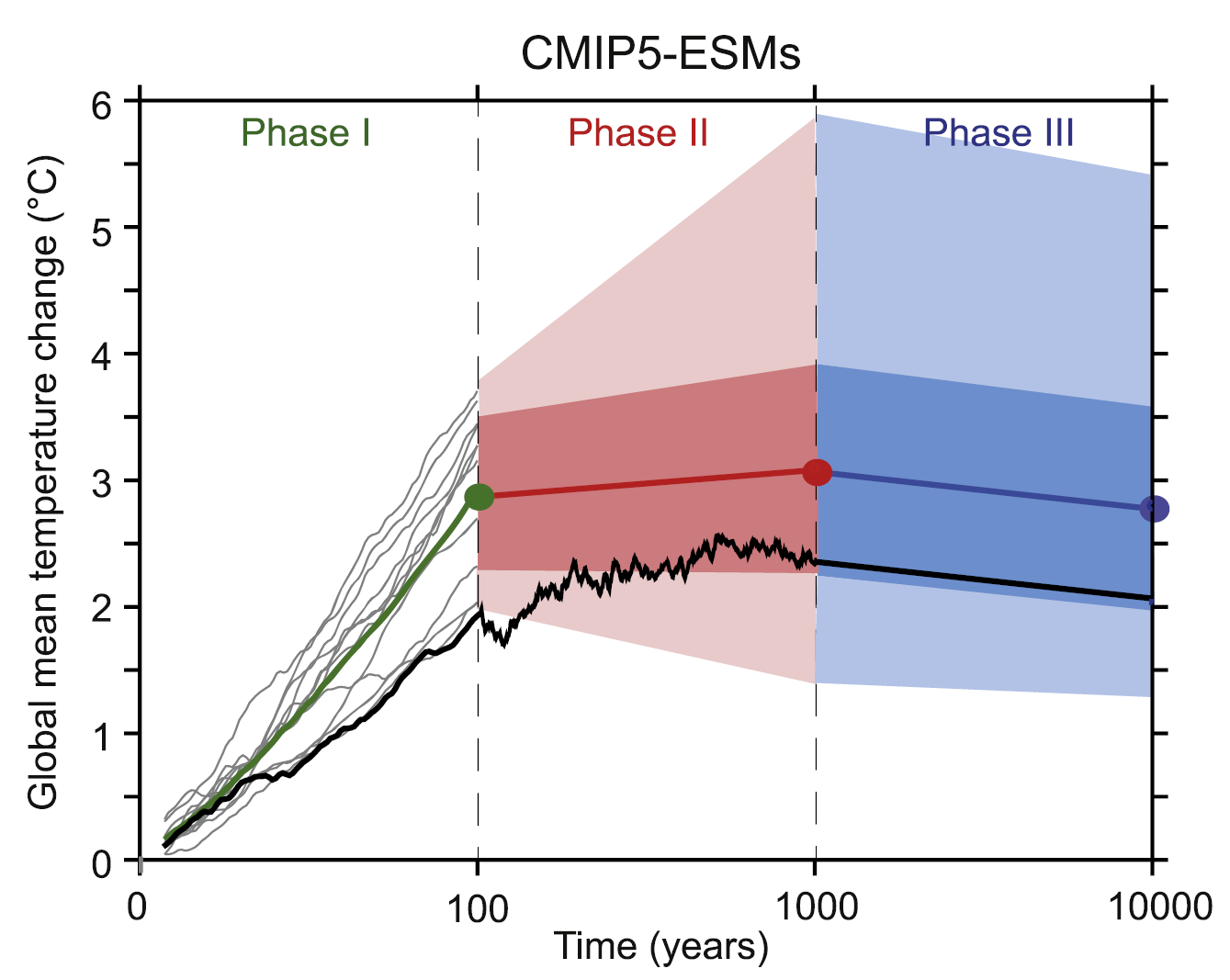
Figure 2. Reproduction of Figure 2.a of Froelicher et al. (2015).3 GMST changes simulated (Phase I) and estimated (Phases II and III) by 12 CMIP5 ESMs.[viii] The multimodel mean is shown by the green/red/blue line. Dark coloured bands show ± 1 standard deviation uncertainty; light coloured bands extend to minimum and maximum model values, both estimated. CO2 is emitted during Phase 1 only, in the amount (varying between models, and averaging 1.9 TtC) needed to increase its atmospheric concentration to 2.7x its preindustrial level by year 100. (The black line, estimated after year 1000, is for the GFDL-ESM2M model, which has a TCRE at the bottom of the range.)
The remarkable stability of GMST in CMIP5 ESMs over a millennium following the cessation of CO2 emissions arises because, in these models, the countervailing effects of ocean absorption of atmospheric CO2 and of ocean heat uptake typically almost cancel out.[ix] The resulting, gradually slowing, decline over time in atmospheric CO2 concentration reduces radiative forcing. Against that, the gradual reduction in the rate of oceanic heat uptake leads to slowly increasing warming for a given level of radiative forcing, as the temperature response to the forcing moves from reflecting the transient climate response (TCR) towards reflecting the higher equilibrium climate sensitivity (ECS) level.[x]
Observationally-based estimates of the transient response to carbon emissions
So much for models and the IPCC’s assessment of TCRE; what do observations indicate? It is fairly straightforward to estimate TCRE from warming and cumulative CO2 emissions to date, but various adjustments need to be made.
According to the HadCRUT4.5 record the GMST increase to the recent decade, 2007-16, was 0.846°C relative to 1850-82, the period from the start of the observational record to just before a period of heavy volcanism. The HadCRUT4 record, however, is not globally complete and may not capture the full global mean increase in surface air temperature, at least in recent years when there was rapid Arctic warming. I therefore use instead the infilled, Cowtan and Way, version of HadCRUT4, which warmed by 0.931°C between the same periods. An alternative way to allow for HadCRUT4’s incomplete global coverage would be to scale 0.846°C up by the ratio of the GMST trend estimated by the globally-complete 1979-on ERA-interim 2 m air temperature measure over 1979-2016, being 0.178°C/decade, to the HadCRUT4.5 trend of 0.173°C/decade over the same period. Doing so would imply an 1850-82 to 2007-16 warming estimate of 0.875°C.
Not all of the observed warming to 2007-16 was due to CO2 emissions. I estimate that total forcing in 2007-16, relative to the mean over 1850-82, was 2.61 W/m2, of which CO2 accounted for 1.67 W/m2, or 64%.[xi] Scaling the observed warming estimate of 0.931°C by 0.64 implies warming in 2007-16 attributable to CO2 emissions averaged 0.596°C. It also implies a TCR estimate of ~1.35°C.
The AR5 estimate of cumulative CO2 emissions over 1750–2011 was 555 GtC. From this, cumulative emissions from 1750 to their 1850-1882 mean, being 31 GtC per the RCP scenarios, need to be deducted in order to compare warming and cumulative emissions over the same period. The difference between average cumulative emissions in 2007–16 and their 2011 value, estimated as 6 GtC,[xii] then needs to be added. That brings the cumulative 1850-82 to 2007-16 total to 530 GtC. However, there is reason to believe that historical CO2 emissions from land-use changes (LUC) are larger than assumed,[xiii] with a suggested underestimation by 35 GtC over 1901-2014.[xiv] Adding this amount would bring the cumulative 1850-82 mean to 2007-16 CO2 emissions to 565 GtC. The observationally-estimated historical TCRE is then simply 0.596 / (565/1000) = 1.05°C.
Observationally-based estimates of the equilibrium response to carbon emissions
Estimating the equilibrium climate response to cumulative emissions is more complicated than estimating the transient response. It requires a simple model that incorporates not only climate system physics but also represents ocean carbonate chemistry and the land biosphere carbon cycle.
The reason why equilibrium warming can in principle be related to cumulative carbon emissions is simple. Unlike other radiatively active-gases in the atmosphere, the timescale on which CO2 is broken down by inorganic chemical reactions (rock weathering) is extremely long – many millennia. On shorter timescales, emitted carbon is simply partitioned between the atmosphere, land ecosystem and ocean. The land ecosystem carbon reservoir will only increase if plant and tree growth is faster, which requires a higher atmospheric CO2 level. The amount of CO2 that can dissolve in the ocean is also directly linked to the atmospheric CO2 concentration. Therefore, although in combination the ocean and land carbon sinks can absorb most of the CO2 emitted into the atmosphere, some of that CO2 must remain in the atmosphere, leaving an elevated concentration. Provided the (temperature-dependent) equilibrium relationships between the increases in the land and ocean carbon reservoirs and the increase in atmospheric CO2 concentration can be satisfactorily approximated, and an estimate of ECS is available, then an estimate of ECRE can be derived.
The simple model I use, which reflects the relevant relationships, is represented by a small number of equations that relate the key variables. I give details of the model equations and the derivation of ECRE in the appendix. The model uses an observationally-based ECS estimate of 1.75°C. The equilibrium ocean and terrestrial ecosystem carbon cycle behaviours of the simple model are both within or at the edge of the EMIC range, which is what the Phase II behaviour in Figure 2 reflects.
The best estimate of ECRE derived from the simple model is 0.5°C.
Based on an ECRE of 0.5°C, if emissions over the 21st century match those in the moderate-mitigation RCP4.5 scenario, which reach 1281 GtC cumulatively over 1765-2100, the equilibrium GMST rise from preindustrial locked in by 2100 would be 0.65°C – lower than current warming, and only a quarter of AR5’s central projection of warming in 2100 under RCP4.5. The corresponding atmospheric CO2 concentration would be 341 ppm, 63 ppm above the preindustrial level, with only 13.5% of the emitted CO2 remaining in the atmosphere. Even assuming that the entire ocean warmed by the full 0.65°C, the ultimate thermosteric rise in sea level – taking a thousand years or more – would be under half a metre.[xv]
Comparing CMIP5 ESM based and observationally-based TCRE and ECRE estimates
The observationally-based TCRE estimate of 1.05°C, although within the AR5 range and the almost identical CMIP5 ESMs model range, is little more than half the level reflected in the central RCP scenario projections in the AR5 SPM.10 chart. Assuming that the 1.05°C estimate is realistic going forward, the IPCC’s chart overstates expected 21st century warming by a factor of approaching two, for all scenarios.
As regards equilibrium warming, while in CMIP5 ESMs the 1000-year ECRE estimate is typically close to the TCRE for the same model, the observationally-based ECRE estimate is only half the observational TCRE estimate.
AR5 Figure SPM.10 projects a broadly linear ratio of multi-model mean warming to cumulative CO2 emissions over the rest of this century, implying that future and historical TCRE are closely aligned. However, the fact that the observationally-based estimate of ECRE is much lower than that of TCRE implies that in the real climate system TCRE is likely to decline over time, so that TCRE estimated from historical observations is likely slightly to overestimate future TCRE. That is because the warming caused by earlier emissions will over time decline from that implied by TCRE towards that implied by the lower ECRE – unlike in the models used by AR5 where ECRE is close to TCRE – which should more than counter the gradual decrease in the ocean’s efficiency at absorbing CO2 as its level of dissolved inorganic carbon increases.
It is pertinent to ask why the ECRE to TCRE estimate ratio based on observational data and a simple model is a factor of two lower than it appears to be in CMIP5 ESMs (Figure 2). There are two reasons. First, the observationally-based estimate of 13.5% of emitted CO2 remaining in the atmosphere after 1000 years is lower than in EMICs (mean 25%, range 17–31%), the carbon-cycle behaviour of which CMIP5 ESMs are assumed to mirror. Secondly, ECS to TCR ratio is much lower for the observationally-based estimates used here: approximately 1.3 compared with an average of 1.8 for CMIP5 models.
Appendix
Estimating the equilibrium climate response to cumulative emissions using observations
I base the required simple model on an established formula that validly reflects ocean carbonate chemistry.[xvi]
ln[pCO2(equil) / pCO2(PI)] ≡ ln[1 + ΔIatmos(equil) / Iatmos(PI)]
= [ΔItotal − ΔIland(equil)] / IB (1)
Equation (1) states that the logarithm of the increase in atmospheric CO2 concentration pCO2 from its initial preindustrial (PI) level to its level in equilibrium after cumulative CO2 emissions of ΔItotal, which is the same as the logarithm of one plus the ratio of the equilibrium increase ΔIatmos in the atmospheric carbon inventory to the initial atmospheric carbon inventory Iatmos, equals the ratio of the excess of total emissions over that part absorbed by the terrestrial ecosystem to the “buffered” carbon inventory IB. AR5 provides a value for preindustrial Iatmos, of 589 GtC.
The buffered carbon inventory equals the carbon content of the atmosphere Iatmos plus the (dissolved) carbon content of ocean Iocean divided by the global mean Revelle or evasion factor R, which represents the buffering arising from ocean carbonate chemistry. AR5 estimates preindustrial IA at 38,000 GtC, while R can be taken from a formula that gives it in terms of the ratio of ΔIocean to Iocean(PI).[xvii] Equation (1) gives more accurate results if, when determining IB, both Iocean and R are taken at their equilibrium rather than their preindustrial values.
I take ECS, on a 1000 year time horizon, as 1.75°C, which is consistent with recent energy budget estimates.[xviii] I allow for climate-carbon feedback arising from the negative effect on the solubility of CO2 in seawater of the rise in ocean temperature (assumed to be 85% of the rise in GMST caused by rising atmospheric CO2 concentration), although it may at least partially be countervailed by increasing efficiency of the ocean biological pump.
It is common to assume that ΔIland is linearly related to ΔIatmos (positively) and to ΔT, the change in GMST (negatively).[xix] The positive influence of ΔIatmos is greatly dominant.[xx] One can therefore estimate the ratio of ΔIland to ΔIatmos for 1000 GtC of cumulative emissions from their relationship from preindustrial to date. AR5 estimated the land sink at 160 GtC over 1750-2011. As that is a balancing figure, the estimated missing LUC emissions of 35 GtC need to be added to it, giving 195 GtC. This is a transient figure, reflecting the effect of CO2 fertilisation on growth of vegetation and the resulting (incomplete) increase in vegetation and soil carbon to date. One can convert it to an equilibrium value by assuming that the terrestrial carbon inventory would decay exponentially in the absence of primary production by photosynthesis, with a fixed time constant corresponding to the average lifetime of carbon in the terrestrial pool. A period of 15-20 years is consistent with what has been assumed elsewhere.[xxi] Modelling, conservatively, on the basis of a 15 year time constant suggests that in 2011 the cumulative land carbon uptake had reached 81% of its eventual, equilibrium, value if atmospheric CO2 concentration remained unchanged thereafter. That implies ΔIland(equilib) = 240 GtC for ΔIatmos(equilib) equal to the increase in atmospheric carbon content up to 2011, of 240 GtC per AR5. That is, ΔIland(equilib) = 1.00 x ΔIatmos.[xxii]
The foregoing relationships, combined with the fact that ΔIocean = ΔItotal – (ΔIatmos + ΔIland), enable a solution that satisfies all the equations to be determined iteratively. The solution implies that 135 GtC out of 1000 GtC CO2 emissions will remain in the atmosphere in equilibrium, producing an increase in concentration of 63 ppm. The ocean absorbs 730 GtC, while the land ecosystem absorbs 135 GtC.
Without any carbon uptake by the land ecosystem and without climate feedback reducing carbon uptake by the ocean, just over 150 GtC would remain in the atmosphere. That is within the 150-210 GtC range projected on the same basis by an ensemble of EMICs.[xxiii] The unit ratio of carbon absorbed by the land ecosystem to that remaining in the atmosphere in equilibrium in the simple model is well within the range projected after 1000 years by an ensemble of EMICs and CMIP5 ESMs.[xxiv]
The radiative forcing resulting from the 63 ppm increase in atmospheric CO2 concentration is 1.1 W/m2. Based on the assumed 1.75°C ECS, the 1.1 W/m2 ultimate increase in CO2 forcing implies that the equilibrium rise in GMST – which by definition is the ECRE – will be 0.5°C.
Nicholas Lewis December 2018
[i] IPCC, 2013: Summary for Policymakers. In: Climate Change 2013: The Physical Science Basis. Contribution of Working Group I to the Fifth Assessment Report of the Intergovernmental Panel on Climate Change [Stocker, T.F.,et al (eds.)]. Cambridge University Press, pp. 1–30.
[ii] Collins, M., and Coauthors, 2013: Long-term climate change: Projections, commitments and irreversibility. Climate Change 2013: The Physical Science Basis, T. F. Stocker et al., Eds., Cambridge University Press, 1029–1136. (Chapter 12 of IPCC AR5 WG1)
[iii] Gillett, N. P., V. K. Arora, D. Matthews, and M. R. Allen, 2013: Constraining the ratio of global warming to cumulative CO2 emissions using CMIP5 simulations. J. Climate, 26, 6844–6858, doi:10.1175/JCLI-D-12-00476.1.
[iv] Approximately 14% of the increase in forcing from 1861-1880 until 1000 GtC emissions are reached arises from non-CO2 sources under RCP4.5 and RCP6.0.
[v] Frölicher, T. L., and D. J. Paynter, 2015: Extending the relationship between global warming and cumulative carbon emissions to multi-millennial timescales. Environ. Res. Lett., 10, 075002, doi:10.1088/1748-9326/10/7/075002.
[vi] ECRE values usually assume cumulative emissions of 1000 GtC, as for TCRE.
[vii] The subsequent slightdecline in GMST (blue line) arises from reactions with calcium carbonate in seafloor sediments removing oceanic dissolved carbon.
[viii] Estimated values for phases II and III use airborne fractions of cumulative carbon emissions simulated by eight EMICs, as hardly any CMIP5 ESMs have carried out actual 1000+ year simulations with a fully-coupled carbon cycle model.
[ix] This occurs despite ocean characteristics varying between models. Such insensitivity to ocean characteristics probably arises because there is much in common between the mechanisms that govern the rates of CO2 and heat transport out of the surface mixed layer into the deeper ocean
[x] TCR represents GMST warming at the end of a 70 year period over which CO2 concentration, rising by 1% p.a., doubles. ECS represents the ultimate GMST increase when CO2 concentration is doubled and then held constant until the atmosphere-ocean system reaches equilibrium. Changes in slow climate system components such as land ice sheets are disregarded.
[xi] These estimates are of effective radiative forcing and are based on IPCC AR5 best estimates up to 2011 save that revised greenhouse gas concentration- forcing relationships (Etminan et al 2016: doi:10.1002/2016GL071930) and post-1990 aerosol and ozone forcing change estimates (Myhre et al. 2017, doi:10.5194/acp-17-2709-2017) have been incorporated. The Etminan et al. CO2 concentration- forcing relationship is also used when calculating what warming a given increase from preindustrial CO2 concentration will produce.
[xii] Global carbon budget 2017. Boden, T. A., Marland, G., and Andres, R. J.: Global, Regional, and National Fossil-Fuel CO2 Emissions, Oak Ridge National Laboratory, U.S.A., 2017; http://cdiac.ess-dive.lbl.gov/trends/emis/overview_2014.html; and average of two bookkeeping models: Houghton, R. A. and Nassikas, A. A.: Global and regional fluxes of carbon from land use and land cover change 1850-2015, Global Biogeochemical Cycles, 31, 456-472, 2017; Hansis, E., Davis, S. J., and Pongratz, J.: Relevance of methodological choices for accounting of land use change carbon fluxes, Global Biogeochemical Cycles, 29, 1230-1246, 2015.
[xiii] Arneth, A., et al, 2017. Historical carbon dioxide emissions caused by land-use changes are possibly larger than assumed. Nature Geoscience, 12, 79-84.
[xiv] It is possible that the underestimation of LUC emissions is overstated, but on the other hand it includes no allowance for possible underestimation prior to 1901. All the 1901-2014 additional LUC emissions are treated as included in the cumulative average for 2007-16. Note that when the additional LUC emissions are included, the (anthropogenic; post 1750) airborne fraction in 2011 is 41%.
[xv] This is based on heat input to the ocean equating to 0.5 W-yr/m2 over the Earth’s surface causing a sea level rise of approximately 1 mm.
[xvi] Goodwin, P. et al, 2007: Ocean-atmosphere partitioning of anthropogenic carbon dioxide on centennial timescales. Global Biogeochem. Cycles, 21, GB1014, doi:10.1029/2006GB002810.
[xvii] Backastow, R, 1981. Numerical evaluation of the evasion factor. In Carbon Cycle Modelling, Scope 16, Bolin, B, ed., John Wiley & Sons, p. 98. Employing instead the function used to relate the partial pressure of CO2 in seawater to its dissolved inorganic carbon content used in the HILDA model (Seigenthaler,U and Joos, F, 1992. Use of a simple model for studying oceanic tracer distributions and the global carbon cycle. Tellus 44B, 186-207) gives an almost identical result.
[xviii] Lewis, N., and J. Curry (2018): The impact of recent forcing and ocean heat uptake data on estimates of climate sensitivity. Journal of Climate 2018. doi.org/10.1175/JCLI-D-17-0667.1 PDF copy here.
[xix] E.g., Friedlingstein, P., 2015. Carbon cycle feedbacks and future climate change. Phil. Trans. R. Soc. A 373.2054: 20140421
[xx] The ratio of ΔT to ΔIatmos will moreover not differ greatly between that to date and that in equilibrium for 1000 GtC of cumulative emissions, on the basis of a TCR of 1.35°C and ECS of 1.75°C.
[xxi] For example, the land biosphere time constant with the largest coefficient in the HILDA model (Joos, F et al 1996. An efficient and accurate representation of complex oceanic and biospheric models of anthropogenic carbon uptake. Tellus 48B 397-417), ignoring two interannual terms, is 20 years.
[xxii] This estimate is consistent, given the adverse relation between ΔIland and ΔT of –28 GtC/°C estimated in Friedlingstein, P (2015) with the (transient) carbon-carbon feedback (CO2 fertilisation strength) estimated in that paper when it is adjusted for the ratio of transient to equilibrium land carbon uptake and for the estimated missing LUC emissions.
[xxiii] Archer et al, 2009. Atmospheric Lifetime of Fossil Fuel Carbon Dioxide. Annu. Rev. Earth Planet. Sci 3 7:117–34
[xxiv] For 100 GtC of emissions, starting from the 2010 CO2 level. Joos et al 2013. Carbon dioxide and climate impulse response functions for the computation of greenhouse gas metrics: a multi-model analysis. ACP, 13, 2793-2825.
Leave A Comment