Committed warming and the pattern effect

A pdf version of this article is available here

A critique of the paper “Greater committed warming after accounting for the pattern effect”, by Zhou, Zelinka, Dessler and Wang.

Key points

The pattern effect is the dependence of outgoing radiation to space on the spatial pattern of surface warming.
A pattern effect, relative to that in equilibrium, can be caused both by evolution over time in the climate system’s response to forcing and by its internal variability.
The paper fails to distinguish between a historical period pattern effect that is forced, which will unwind very slowly, and one that is caused by internal variability, which can quickly unwind, causing rapid warming.
The forced pattern effect is very small in CAM5.3
The pattern effect found in the paper is greatly affected by being estimated during the hiatus.
The estimated post-hiatus unforced historical pattern effect is non-negligible in CAM5.3 when using the AMIP2 sea surface temperature dataset, as in the paper, but negligible when using the UK Met Office HadISST1 dataset.
The historical pattern effect is not robust; it varies hugely between models and SST datasets.
The paper’s claims about greater committed warming directly reflect its estimate of the size of the historical pattern effect.

Introduction

A new paper “Greater committed warming after accounting for the pattern effect” led by Chen Zhou (Zhou et al.[1]) has recently been published in Nature Climate Change. Here is the accompanying press release.

Zhou et al.’s estimate of committed warming (future warming with forcing remaining unchanged) follows fairly directly from their estimate of the pattern effect, if one accepts their bases and assumptions. In this article I therefore mainly deal with their estimate of the pattern effect.

The term “pattern effect” refers to the effect on outgoing radiation to space of the spatial pattern of surface temperatures, with unchanging global mean temperature. Mauritsen (2016)[2] gives a simple explanation of how the pattern effect arises. The effect implies that, in the global mean, climate feedback strength – the ratio of the global change in outgoing radiation to that in surface temperature –depends on the spatial pattern of evolving surface temperature change.

In numerical value terms:

Pattern effect = Actual net outgoing radiation to space – Expected long term mean outgoing radiation (at the applicable global mean surface temperature)[3]

where

Expected long term mean outgoing radiation = Increase in global temperature from previous equilibrium state × Long term climate feedback strength under increased CO₂

It follows that climate sensitivity estimates derived from the change in global temperature and the Earth’s energy balance over the historical period (since 1850 or so) are potentially subject to bias if the pattern of surface temperature change over the historical period differs from the long term pattern of warming arising from increased CO₂ concentration, which is what will determine equilibrium climate sensitivity.

Unfortunately, the pattern effect – most importantly, its evolution over the historical period – can only be quantified using global climate model (GCM) simulations, in atmosphere-only mode. Those simulations (amipPiForcing simulations), although driven by observational sea surface temperature (SST) and sea-ice data, are quite strongly dependent both on individual model characteristics and on the evolution of SST in regions that historically have been sparsely observed.

There is nothing fundamentally new in Zhou et al.’s paper about the pattern effect and its implications for bias in observationally-based estimates of climate sensitivity and for ultimate future warming. The pattern effect has been known about for several years, and its potential implications for historical period observational estimates of climate sensitivity discussed, for example in Lewis and Curry (2018)[4]. Moreover, Andrews et al. (2018)[5] carried out a very similar analysis to that in the new paper. Although Zhou et al. and Andrews et al. (2018) use somewhat different models and analysis methods, there is little difference in their estimates of the historical period pattern effect. However, historical period pattern effect estimates vary greatly according to the climate model and SST dataset involved, and are not robust.

The total pattern effect arises from the sum of two distinct influences on surface temperature patterns:

the evolution over time in the spatial pattern of the climate system’s forced response to increased CO₂ forcing, which causes climate feedback strength in the long term to differ from that over the shorter term, such as the historical period; and
the effect of climate system internal variability on temperature, particularly SST, patterns

which give rise to respectively the forced and unforced pattern effects.

The importance of distinguishing between forced and unforced pattern effects

A serious shortcoming in both Andrews et al (2018) and Zhou et al (2021) is that they only estimate the total pattern effect.[6] But its forced and unforced components have very different implications for the timescale over which future warming develops.

The forced pattern effect is very difficult to identify in observations, however it occurs in a large majority of coupled GCMs[7] in simulations driven by increased CO₂ concentration. Within a decade after such an increase, their surface warming patterns change and their climate feedback strength starts to decline to a somewhat lower level. Therefore, coupled GCM’s long term climate feedback strength is overestimated, and their equilibrium climate sensitivity (ECS) underestimated, if based on data from the early decades after an increase in CO₂ concentration – which broadly corresponds to data available from the historical period.

Nevertheless, if there were only a forced pattern effect over the historical period, then coupled GCM behaviour implies that use of ‘effective climate sensitivity’ estimates that correctly reflect warming and energy budgets over the historical period can be expected to result in very little underestimation of committed warming up to 2100,[8] or until the mid-2100s for warming from increases in forcing between now and then, with underestimation only emerging slowly thereafter.[9]

However, if there were also a non-negligible positive unforced pattern effect component over the historical period, then as soon as the internal variability excursion causing it ends, global mean temperature would rapidly increase. Moreover, historical period ‘effective climate sensitivity’ estimates would be further biased low. Therefore, using them could significantly underestimate both committed warming and warming from future forcing increases over the current century, not just in the longer run as for a forced pattern effect.

Since forced and unforced pattern effects have very different implications for the timescale of future warming, it is important to produce separate estimates of their magnitudes over the historical period.

Lewis and Mauritsen (2020)[10] showed that the estimated magnitude of the historical period unforced pattern effect is strongly dependent, in at least one model[11], on the observational SST dataset used. We found it to be significant when employing AMIP2 SST, as is usual in the SST-driven climate model simulations involved, but negligible when UK Met Office HadISST1 SST data was employed.[12]

In my view, the most useful contribution of Zhou et al (2021) is this. They carried out simulations with another model, CAM5.3, driven by HadISST1 SST data as well as by the usual AMIP2 SST data. They also performed an abrupt4xCO2 simulation for CAM5.3 in coupled mode. In this article, I will show what the implications of their CAM5.3 simulations are for the forced pattern effect and – based on each of AMIP2 and HadISST1 SST data – for the unforced historical pattern effect.

The forced pattern effect in CAM5.3: how does its climate sensitivity change over time?

Standard practice is to estimate the ECS of a coupled GCM by running a simulation under preindustrial conditions until a near-equilibrium state is reached, and then performing a 150 year long simulation at the start of which the CO₂ concentration is quadrupled (‘abrupt4xCO2’). Usually ECS is estimated from the x-intercept of a linear OLS[13] regression fit of top-of-atmosphere radiative imbalance (global heating rate, N) to global near-surface air temperature (T), both expressed as annual mean changes from their preindustrial mean[14]. The x-intercept value, which corresponds to a stable state with zero net heating, is generally halved to convert from a quadrupling of CO₂ concentration to the doubling specified for ECS.[15] The climate feedback parameter (λ) is taken as the negative of the regression fit line’s slope.[16]

When estimating feedbacks in amipPiForcing simulations there are good arguments for using surface temperature (Ts – SST over ocean and land skin temperature) rather than near-surface air temperature (Lewis and Curry 2018). Zhou has previously done so, and I do so here. The effect of such blending of temperature measures is extremely small in CAM5.3; Ts increases by 1.0% less than T over the abrupt4xCO2 simulation, implying an ECS of 2.97 K rather than 3.00 K per Zhou et al.

Figure 1 shows the CAM5.3 abrupt4xCO2 simulation annual Ts and N values (blue line).[17] The leftmost end of the line shows the year 1 mean values. The red line shows the linear fit over years 1-150 and resulting ECS estimate. Its slope implies λ = 1.32 Wm⁻²K⁻¹; the x-intercept of 5.94 K corresponds to an ECS of 2.97 K when halved.

In order to estimate the forced pattern effect for CAM5.3, one also needs an estimate of its climate feedback value that would have been applicable over the historical period. This can be estimated from the slope of a regression fit over the first twenty to fifty years of its abrupt4xCO2 simulation.

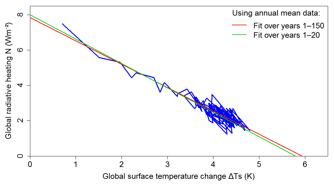
Figure 1. Plot of annual mean ΔTs and N values over the 150 year CESM1.2.1-CAM5.3 abrupt4xCO2 simulation, and linear OLS regression fits thereto over years 1–150 and 1–20. The x-intercepts of approximately 6 K imply an ECS of 3 K (from the years 1–150 fit line) and a marginally lower effective climate sensitivity estimate (from the years 1–20 fit line), if halved to convert from 4× CO₂ to 2× CO₂ (as is usually done). The climate feedback parameter, λ, estimates over years 1–150 and 1–20 are the negatives of the relevant regression line slopes.

Examination of the amipPiForcing data suggests that fitting a regression over the first twenty years would be more appropriate here. Doing so (green line in Figure 1) gives a 4.5% higher λ estimate, of 1.38 Wm⁻²K⁻¹, than regression over years 1–150; the resulting effective climate sensitivity estimate of 2.90 K is just 2.4% smaller than the ECS estimate.[18]

I use the 0.06 Wm⁻²K⁻¹excess of the climate feedback estimate from regressing abrupt4xCO2 data spanning years 1–20 (λ₂₀) over that from regressing data spanning years 1–150 (λ₁₅₀) as the best estimate, in λ terms, of the forced pattern effect applicable to the historical period in CAM5.3. The forced pattern effect on outgoing radiation is then obtained as:

Forced pattern effect = (λ₂₀– λ₁₅₀) × Change in surface temperature (1)

Zhou et al. also mention, but do not explore, the possibility of estimating the (total) pattern effect using a long term λ value calculated using years 21–150 rather than 1–150 abrupt4xCO2 data. Issues when estimating such a λ value are discussed in an Appendix to this article.

The unforced pattern effect in CAM5.3

Zhou et al. estimate the total pattern effect over the historical period by comparing outgoing radiation with surface air temperature change, based on CAM5.3 amipPiForcing simulations driven by AMIP2 SST and sea-ice data, as is standard for such simulations. However, they also perform such simulations driven by HadISST1 SST data.

Zhou et al. estimate the total pattern effect using a long term climate feedback parameter, estimated over years 1–150 of the abrupt4xCO2 simulation, λ₁₅₀. I do the same as them to estimate the unforced pattern effect over the historical period, but using a climate feedback parameter estimated over years 1–20 of the CAM5.3 abrupt4xCO2 simulation, λ₂₀, which appropriately represents the model’s forced response during the historical period.

Total pattern effect = Change in outgoing radiation – λ₁₅₀ × Change in surface temperature (2)

Unforced pattern effect = Change in outgoing radiation – λ₂₀ × Change in surface temperature (3)

Figure 2 shows how the unforced pattern effect (unforced outgoing radiation) varies during the CAM5.3 amipPiForcing AMIP2 and HadISST1 based simulations; 3-year year running means are plotted as doing so produces a clearer comparison.[19] It can be seen that until just after 1980 the two datasets produce quite similar pattern effects. That is as expected, because the AMIP2 dataset uses HadISST1 sea-ice data (with minor adjustments) throughout the historical period, and uses HadISST1 SST data until 1981, albeit with an altered anomalisation pattern.[20] However, from late 1981 on AMIP2 uses a different SST dataset and the pattern effect estimates diverge substantially. Both datasets produce a positive pattern effect from the late 1990s on, but its magnitude is far larger using the AMIP2 dataset.

Zhou et al.’s main estimate of the total pattern effect, of 0.63 Wm⁻², uses AMIP2 data and is based on the mean over the five year period 2006–2010.

Although I use surface temperature (Ts) not surface air temperature (T) data, when using AMIP2 data I obtain an identical 0.63 Wm⁻²estimate for the total pattern effect over that period, and a 0.59 Wm⁻²estimate for the unforced pattern effect (horizontal red line in Figure 2).[21]

However, based on HadISST1 SST data, the unforced pattern effect estimated over 2006–2010 is little more than half that based on AMIP2 data, at 0.34 Wm⁻²(horizontal blue line in Figure 2).

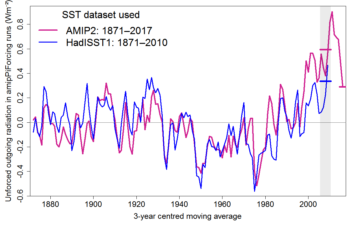
Figure 2. Plot of 3-year running average of estimated annual mean unforced outgoing radiation over the historical period, based on ensemble means from three CAM5.3 amipPiForcing simulation runs each driven by either AMIP2 data (red line) or HadISST1 SST data (blue line). The values plotted are global outgoing radiation to space minus the product of global surface temperature and the climate feedback parameter estimated over years 1–20 of the CAM5.3 abrupt4xCO2 simulation, as anomalies relative to the 1871–1880 means. Colour-matching horizontal lines show means of annual data over 2006–2010 for simulations based on both datasets, and over 2015–2017 for AMIP2-based simulations; the HadISST1-based simulation ends in 2010.

The distorting effect of the Hiatus

Although Zhou et al. performed simulations based on AMIP2 – their primary dataset – extending to 2017, they used 2006-2010 as the period over which to estimate the pattern effect for CAM5.3.[22] However, 2006–2010 is not very representative of the historical period since it falls within the last ‘hiatus’, during which global temperature increased much less that was expected given the continuing strong increase in greenhouse gas concentrations. The most convincing explanations of the hiatus involve unusual conditions in the Pacific area caused by strong decadal internal variability, which for about a decade suppressed warming without a commensurate reduction in outgoing radiation. Cooling in the eastern Pacific relative to the west Pacific warm pool, as occurred in the hiatus, and the associated increase in low cloud cover in the eastern Pacific and other tropical areas, is expected to increase outgoing radiation. In other words, internal variability caused a positive pattern effect during the hiatus.

The estimated post-hiatus unforced pattern effect

AMIP2-based

Since Zhou’s AMIP2-based amipPiForcing simulation extends to the end of 2017, and the hiatus was over by the end of 2014, one can form an AMIP2-based estimate of the post-hiatus pattern effect magnitude by taking its mean over 2015–2017.[23] Although this is an even shorter averaging period than used by Zhou et al. (3 rather than 5 years), the estimation uncertainty should not be hugely greater.[24] Over 2015–2017, the estimated AMIP2-based unforced pattern effect is 0.29 Wm⁻² (rightmost horizontal red line in Figure 2), 0.30 Wm⁻² lower than that over 2006–2010.

HadISST1-based

Unfortunately, Zhou chose not to continue his HadISST1-based amipPiForcing simulation beyond 2010. However, it appears that the divergence between the AMIP2- and HadISST1-based unforced pattern effect estimates very largely arose in the later part of the 20th century; it is unconnected with the hiatus. Since the mid-1990s the difference between them has been fairly stable, albeit fluctuating. There is almost no trend in the difference over either the ten or fifteen years to 2010.[25] One can therefore use the difference between the AMIP2-based unforced pattern effect estimates over 2006–2010 and over 2015–2017 as a proxy for the corresponding difference for HadISST1-based estimates. Doing so implies a HadISST1-based post-hiatus unforced pattern effect estimate over 2015–2017 of merely 0.04 Wm⁻². This is negligible, and far below estimation uncertainty.[26]

Conclusions

Zhou et al.’s pattern effect estimates are applicable only to the unusual hiatus period. Insofar as historical period climate sensitivity estimates are dominated by the hiatus period, it might nevertheless be reasonable to use them when estimating the effect on committed warming since early industrial times. However, previous studies have found little difference between energy budget climate sensitivity estimates formed using different periods, or using regression over the full period (Lewis and Curry 2015[27], Lewis and Curry 2018, Otto et al. 2013[28]). Moreover, Lewis and Mauritsen (2020) found a negligible unforced pattern effect when estimating it by regression using HadISST1 data over 1871–2010 period.

Zhou et al.’s focus on AMIP2 SST based pattern effect estimates, which are much higher than those derived using HadISST1 data, is unfortunate. AMIP2 is a merged dataset and, after 1981, uses SST data derived using an interpolation method that is arguably less suitable for estimating the pattern effect than the method used by HadISST1 (Lewis and Mauritsen 2020).

When HadISST1 SST data are used, the estimated post-hiatus unforced pattern effect is negligible. On that basis, committed future warming accounting will be almost unaffected by the pattern effect over the rest of this century, since the forced pattern effect only increases warming very slowly[8]. Use of ‘effective climate sensitivity’ estimates that correctly reflect warming and energy budgets over the full historical period, and are not unduly influenced by the hiatus, can accordingly be expected to result in very little underestimation of committed warming up to 2100, at least, if GCM amipPiForcing simulations based on HadISST1 data are a guide..

When AMIP2 SST data are used, there is a non-negligible (but of uncertain significance) estimated post-hiatus unforced pattern effect, but it is only half the magnitude of that estimated over 2006-2010, the period used by Zhou et al.

Appendix: ECS estimation in abrupt4xCO2 simulations and pitfalls of using annual mean data

Zhou et al. point out that a long term λ value derived from regressing over years 21–150 rather than 1–150, which there is a case for and is sometimes done, would be smaller and hence produce a larger estimate of the (forced element of the) historical pattern effect. However, a model’s interannual internal variability (particularly evident in Figure 1after the first 20 years or so) can noticeably bias the slope estimate over years 21–150 of abrupt4xCO2 data if annual means are used, if its climate feedback for interannual variability differs from that to CO₂ forcing over the analysis period. It is therefore better practice to regress pentadal or other multiyear mean data to estimate λ over years 21–150.

Figure 3 repeats Figure 1 but using pentadal rather than annual mean data. It can be seen just how linear the CAM5.3 model behaviour is once the effects of interannual variability are dampened. The years 1–150 and 1–20 regression slopes (and hence λ estimates) are both about 4%–5% smaller than when using annual mean data. However, the ECS and effective climate sensitivity estimates are barely changed; the latter is now only 1% (rather than 2.4%) below the ECS estimate.

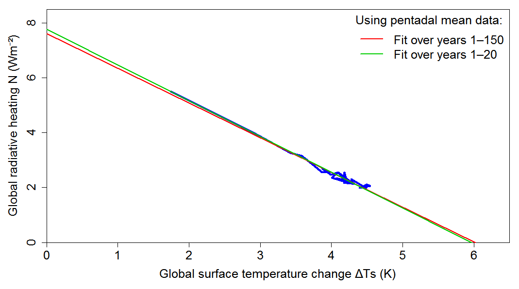
Figure 3. Plot of pentadal mean ΔTs and N values over the 150 year CESM1.2.1-CAM5.3 abrupt4xCO2 simulation, and linear OLS regression fits thereto over years 1–150 and 1–20.

Regressing over pentads formed for years 21–150 data would give an ECS estimate 6.4% higher than that using years 1–150 data (fit line not shown), and a substantially smaller λ estimate. However, if years 21–150 pentadal data were regressed the other way around (ΔTs on N, not N on ΔTs) then the ECS estimate would be less than 1% above that using years 1–150 data, and the λ estimate would be considerably closer to that using years 1–150 data. When annual mean data is regressed, the difference in λ estimates over these two periods depends to a much greater extent on which way round the regression is performed. The substantially larger impact on regression over years 21–150 than over years 1–150 of random variability in Ts (or T) and N, results from the forced change being much lower over that period. That results in lower data correlation. Using pentadal rather than annual means substantially improves the forced-signal-to-noise ratio and hence the data correlation and regression accuracy.

Even when pentadal means are used, there is some uncertainty in the ECS estimate, and large uncertainty in the λ estimate, when using data spanning years 21–150. By contrast, when using years 1–150 data ECS estimation is almost unaffected, and λ estimation is affected by under 3%, by which way round the regression is performed when using pentadal mean data (although the way round regression is performed does noticeably affect both ECS and λ estimates when using annual mean data).

Nicholas Lewis 19 January 2021

[1] Zhou, C., Zelinka, M. D., Dessler, A. E., & Wang, M., 2021: Greater committed warming after accounting for the pattern effect. Nature Climate Change, 1-5. https://doi.org/10.1038/s41558-020-00955-x

[2] Mauritsen, T., 2016. Clouds cooled the Earth. Nature Geoscience, 9(12), pp.865-867. https://www.nature.com/articles/ngeo2838/

^[3] Zhou et al. define the pattern effect the same way but with the opposite sign. Since the pattern effect is the effect of surface warming patterns on outgoing radiation, my sign convention seems more natural.

^[4] Lewis, N. and J. Curry, 2018: The Impact of Recent Forcing and Ocean Heat Uptake Data on Estimates of Climate Sensitivity. J. Climate, 31, 6051–6071, doi.org/10.1175/JCLI-D-17-0667.1.

^[5] Andrews T et al., 2018 Accounting for changing temperature patterns increases historical estimates of climate sensitivity. Geophys. Res. Lett. 10.1029/2018GL078887

^[6] I critiqued Andrews et al. (2018) in an earlier article, partly for the failure to distinguish between the two types of pattern effect. https://nicholaslewis.org/warming-patterns-are-unlikely-to-explain-low-historical-estimates-of-climate-sensitivity/

^[7] An atmospheric GCM coupled to a dynamic ocean model, being an AOGCM. The coupled version of CAM5.3 used by Zhou et al. is CESM1.2.1-CAM5.3. GCMs can also be run in atmosphere-only mode (AGCMs), with externally provided SST and sea-ice boundary conditions. That is what is done in AMIP simulations, including amipPiForcing simulations.

^[8] Mauritsen, T., and R. Pincus, 2017: Committed warming inferred from observations. Nat. Climate Change, 7, 652–655, https://doi.org/10.1038/nclimate3357.

^[9] No such underestimation should arise if using historical period observational estimates of climate sensitivity that adjusted for the forced pattern effect found in coupled GCMs, as presented in Lewis & Curry (2018) and some other studies.

^[10] Lewis N, Mauritsen T. Negligible unforced historical pattern effect on climate feedback strength found in HadISST-based AMIP simulations. Journal of Climate. 2020 Nov 24;34(1):39-55. https://doi.org/10.1175/JCLI-D-19-0941.1

^[11] In ECHAM6.3, and its coupled version MPI-ESM1.1.

^[13] OLS: ordinary least squares

^[14] Sometimes adjusted for drift occurring during the preindustrial control run.

^[15]Doing so overestimates ECS by almost 5%, as CO2 radiative forcing increases slightly faster than logarithmically with concentration.

^[16] I define λ as the change in net outgoing radiation with surface temperature, as in the last IPCC report, which matches the sign convention in Lewis and Mauritsen (2020) and Zhou et al; Andrews et al (2018) use the opposite convention.

^[17] As I do not currently have data for the CAM5.3 piControl simulation, I have derived the preindustrial mean Ts value from the ECS value stated in Zhou et al., on the assumption that the piControl simulation was stable, with zero N.

^[18] Regressing instead over years 1–50 would give a marginally higher λ estimate of 1.396 Wm−2K−1.

^[19] All values are anomalies relative to 1871–1880 means, the reference period used by Zhou et al.

^[20] See Lewis and Mauritsen (2020) for further details of the construction of both the HadISST1 and the AMIP2 SST datasets.

^[21] Since in the AMIP2 (and the HadISST1) amipPiForcing simulations the rise in Ts to 2006–2010 was 0.6 K, the 0.06 Wm−2 K−1 forced pattern effect component of the total pattern effect amounts to 0.04 Wm−2 over 2006–2010.

^[22] To be fair, Zhou may well have done so in order to show comparisons with existing amipPiForcing simulations by other GCMs that ended in 2010.

^[23] Zhou et al. do give, in their Methods section, an estimate of the AMIP2-based pattern effect over 2011–2017, but the hiatus continued during first few years of that period.

^[24] For independent random variables, averaging over 3 rather than 5 realisations would increase uncertainty by 29%. A rough measure of the increase in uncertainty in this case can be obtained by comparing the standard deviation of detrended 3-year mean and pentadal mean estimates of the pattern effect over 1871-2010. That suggests no more than a 15% increase in uncertainty.

^[25] The trends in the AMIP2 minus the HadISST1 annual pattern effect estimates was –0.001 Wm−2 year −1 over 1996-2010 and –0.009 Wm−2year−1 over 2001-2010.

^[26] Zhou et al. put uncertainty at ± 0.27 Wm−2 for their main 5-year mean 2006–2010 AMIP2-based pattern effect estimate of 0.63 Wm−2.

^[27] Lewis, N., and J. A. Curry, 2015: The implications for climate sensitivity of AR5 forcing and heat uptake estimates. Climate Dynamics, 45(3-4), 1009-1023. https://doi.org/10.1007/s00382-014-2342-y.

^[28] Otto, A. and Coauthors, 2013: Energy budget constraints on climate response. Nature Geosci., 6, 415–416. https://doi.org/10.1038/ngeo1836.

Committed warming and the pattern effect