Originally a guest post 31 October 2019 at Climate Audit
Introduction
The recent open-access paper Gregory et al 2019 “How accurately can the climate sensitivity to CO2 be estimated from historical climate change?” discusses, inter alia, the use of regression to estimate historical climate feedback. As I wrote in a previous article, Gregory et al. consider a regression in the form R = α T, where T is the change in global-mean surface temperature with respect to an unperturbed (i.e. preindustrial) equilibrium and R is the radiative response of the climate system to the change in T, however caused; α is thus the applicable climate feedback parameter for that cause. The corresponding effective climate sensitivity (EffCS) is then F2xCO2/α where F2xCO2 is the effective radiative forcing (ERF) for a doubling of preindustrial atmospheric carbon dioxide concentration. It should be noted that the climate system response to ERF, in GCMs and/or the real world, may vary between forcing agents: their (equilibrium) efficacies[1] may differ or, equivalently, different α values may apply to them. This is thought to be a major issue in relation to volcanic forcing, at least.[2] [3]
Gregory et al. go on to consider time-variation of climate feedback in the standard CMIP5 climate model historical experiment simulations spanning 1850-2005 featured in AR5. They attempt to do so for the AR5 CMIP5 models generally. This a very difficult task, since ERF was not generally diagnosed for CMIP5 historical simulations, and evidently varies very substantially between models. An accurate ERF time series is needed in order to derive one for R, using R = ERF – N (where N is the Earth’s downwards top-of-atmosphere (TOA) radiative imbalance) since R cannot be measured directly in models or in the real world. As a surrogate for evolving CMIP5-mean historical simulation ERF, Gregory et al. use IPCC AR5 estimated total ERF, with the anthropogenic aerosol component multiplied by 1.5 and the volcanic component multiplied by 0.8 to compensate for estimated differences between CMIP5 and AR5 historical ERF. My investigations suggest that doing so, which undoubtedly better than using unadjusted AR5 ERF, does not provided a sufficiently accurate match to the time profile of CMIP5-mean historical simulation ERF evolution. I do not think that there is any fully satisfactory way of resolving this problem.[4]
Gregory et al. analyse the data using ordinary least squares (OLS) regression of R against T during the historical period over sliding 30-year windows, and conclude that the level of climate feedback (α: the slope of this regression) varies substantially in AOGCM historical simulations on multidecadal timescales, by a factor of up to two. Figure 1 reproduces the relevant figure in their paper. The solid black line shows how estimated α varies when regressing CMIP5 multimodel-mean historical simulation data, using their surrogate ERF time series. The dotted black line is the mean of α estimates for individual CMIP5 model-ensembles (each comprising from one to ten runs), with the shaded area showing ±1 standard deviation bounds. As Gregory et al. correctly point out, due to “regression dilution” use of OLS regression biases α estimates downwards in the presence of noise in the explanatory variable, T. Such noise is much greater for individual models than for the CMIP5 multimodel-mean, where it averages out much more.
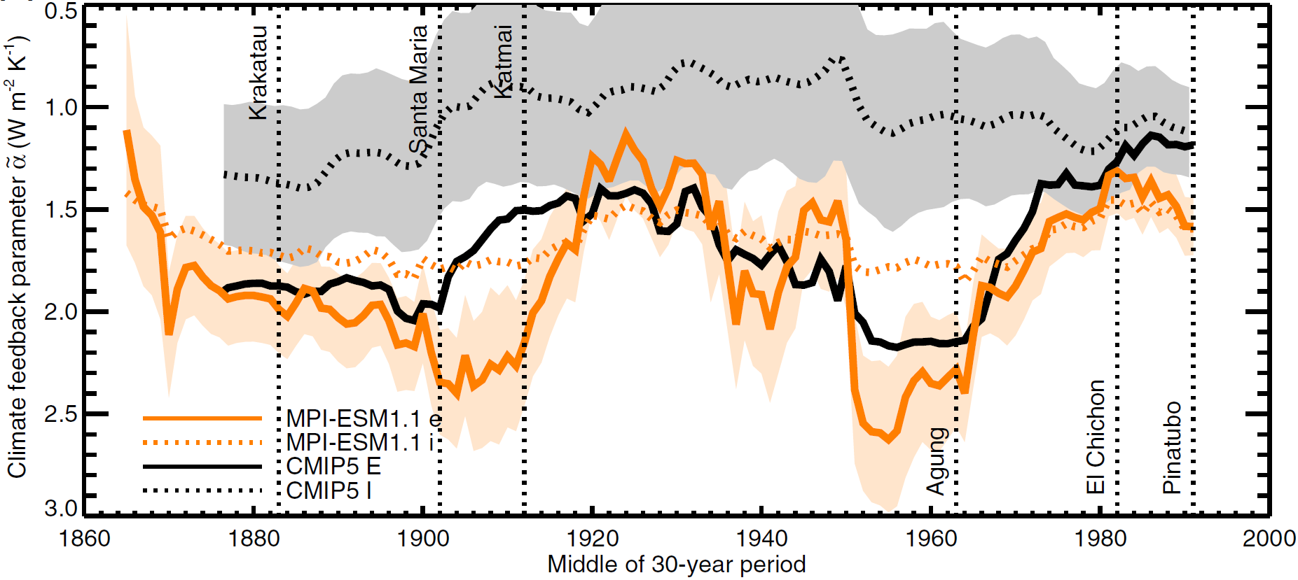
Figure 1. A reproduction of Fig. 5(a) in Gregory et al (2019). Time-dependent climate feedback parameter for the multimodel mean of the CMIP5 historical experiment (labelled“CMIP5 E”) compared with the mean ‑I of individual CMIP5 models (labelled “CMIP5 I”), and corresponding ‑e and ‑i from the MPI-ESM1.1 ensemble. The lightly coloured regions around the CMIP5 I lines are ±1 standard error.
I do not suggest here that anything in this part of the new paper is wrong. Moreover, Gregory et al. correctly state a key point, that the time-variation of α estimated for the CMIP5 mean can be explained mainly by the varying importance of greenhouse gas and volcanic forcing. However, I think that climate feedback estimates derived from 30 years of historical period data, with no adjustment in relation to volcanic forcing, are not the best method of analysis. Such regressions reflect noise from internal climate system variability and the low efficacy (or, equivalently, the high α) of volcanic forcing. But, even assuming accurate ERF estimates are used, the 30-year sliding regression analysis does not reveal what, if any, non-noise caused variability in α remains after adjustment is made for the low efficacy of volcanism. I focus here on the use of an alternative method of analysis that I believe provides more insight into climate model behaviour during historical simulations.
Analysing climate feedback in MPI-ESM1.1
In addition to looking at AR5 CMIP5 models, Gregory et al. sensibly investigated the ensemble of CMIP5-style historical simulations carried out by the Max Plank Institute in Hamburg using their more recent MPI-ESM1.1 AOGCM. That ensemble is ideal for investigating α estimates, both because it has far more members (100) than other ensembles of multiple historical simulations and, even more so, because related diagnostic simulations that enable accurate quantification of the ERF applying in each year of the historical simulation have also been carried out with this model. As the solid orange line in Figure 4 shows, on Gregory et al.’s chosen method of 30-year regression analysis α varied even more over the historical period for the MPI-ESM1.1 ensemble mean than for the CMIP5 multimodel-mean.
The paper states that the distribution of estimated climate feedback obtained by OLS regression of R against T over the 100 individual MPI-ESM1.1 full historical simulation runs is 1.38±0.08 Wm−2K−1 (mean and standard deviation), and that this is consistent with the median of 1.43 Wm−2K−1 estimated by Dessler et al. (2018)[5] from the same dataset using differences between the means of the last and the first decades
However, the diagnosed forcings for 1851 and, particularly, 1850, were affected by spin-up issues (Thorsten Mauritsen, oral personal communication 8 August 2018).[6] When omitting these years from the period analysed, the median α estimates from differencing averages of the last and first decades and from OLS regression are closer, at 1.34 and 1.37 Wm−2K−1 respectively. However, the regression estimate will inevitably be affected by the response to episodic volcanic forcing differing from that to other forcings, as will the differencing method in this case since volcanic forcing differed materially between 1852-1861 and 1996-2005. While – as the paper says – due to using more data regression gives a smaller slope uncertainty than the differences-of-means method, this advantage becomes smaller if longer averaging periods are used. Differencing between averages over 20 years reduces the standard deviation of the slope (α) estimate to under 0.10 Wm−2K−1, little more than the 0.08 Wm−2K−1 for regression.
Unfortunately, the raw diagnosed MPI-ESM1.1 historical simulation ERF estimates are biased low. That is because they are derived from the changes in TOA radiative imbalance in simulations by the model’s atmospheric component (ECHAM6.3) with the same changes in atmospheric composition and land use as in the historical simulation but fixed sea surface temperatures (SST). The land surface warms in these fixed SST simulations, but no correction was made here for the resulting increase in R, resulting in underestimation of the historical simulation ERF. This is a well known issue, but it is usually ignored.[7] Scaling the unadjusted historical ERF by a factor of 1.07 provides an appropriate correction for land surface warming.[8] When this correction is made, and additionally the model’s response to volcanic forcing is allowed to differ from that to other forcings, the 1.37 Wm−2K−1 α regression estimate from ensemble-mean 1852-2005 historical simulation data becomes 1.45±0.035 Wm−2K−1.[9]
The method I use to adjust for the different efficacy of volcanic forcing is to include the AR5 volcanic forcing series as a separate regressor (explanatory variable); its estimated regression coefficient is 0.15±0.02. Since the AOGCM’s diagnosed volcanic ERF is only about 80% as high as volcanic forcing per AR5,[10] that implies that the equilibrium efficacy of volcanic ERF in MPI-ESM1.1 is approximately (0.8 – 0.15) / 0.8, or 0.8. Equivalently, one could say that α for volcanic ERF is some 1.25x that for CO2 and other historical forcing agents. This method introduces one additional free parameter, which due to the episodic nature of volcanism can be well estimated. The single α estimate produced by this approach applies to the sum of non-volcanic ERF and efficacy-scaled volcanic ERF, not to their unweighted sum.
When further adjusting the diagnosed historical ERF for the low efficacy of volcanic forcing, by deducting AR5 volcanic forcing scaled by the 0.15 regression coefficient estimate, α estimates from taking the ratio of differences in mean R and T between averages for the last and first one, two or three decades are 1.44–1.45 Wm−2K−1, essentially identical to the regression derived estimate.
Importantly, when the low efficacy of volcanic forcing is allowed for by including AR5 volcanic forcing as well as T a regressor when regressing MPI-ESM1.1 historical simulation annual ensemble mean land-surface warming adjusted R over 1852-2005, there is no evidence of any time variation in α whatsoever. Figure 2 shows the fit between the diagnosed historical ERF, corrected for land surface warming and adjusted for the low equilibrium efficacy of volcanic forcing, and ERF estimated from ensemble-mean changes in T and in TOA radiative imbalance N in the MPI-ESM1.1 historical simulations, based on the α estimate of 1.45 Wm−2K−1.[11] The fit is excellent, with a regression R2 of 0.93 (0.96 correlation). Note that the residuals will reflect any time variation in the efficacy of volcanic ERF as well as any time variation in α.
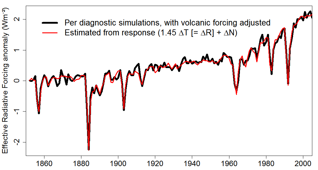
Figure 2. Diagnosed 1852-2005 historical ERF for MPI-ESM1.1, when land-surface warming and the low efficacy of volcanic forcing are adjusted for, and that estimated from the model’s ensemble-mean historical simulations response using a fixed 1.45 Wm−2K−1 climate feedback (α) estimate.
The residuals from the fit (Figure 3) appear random and have low autocorrelation.
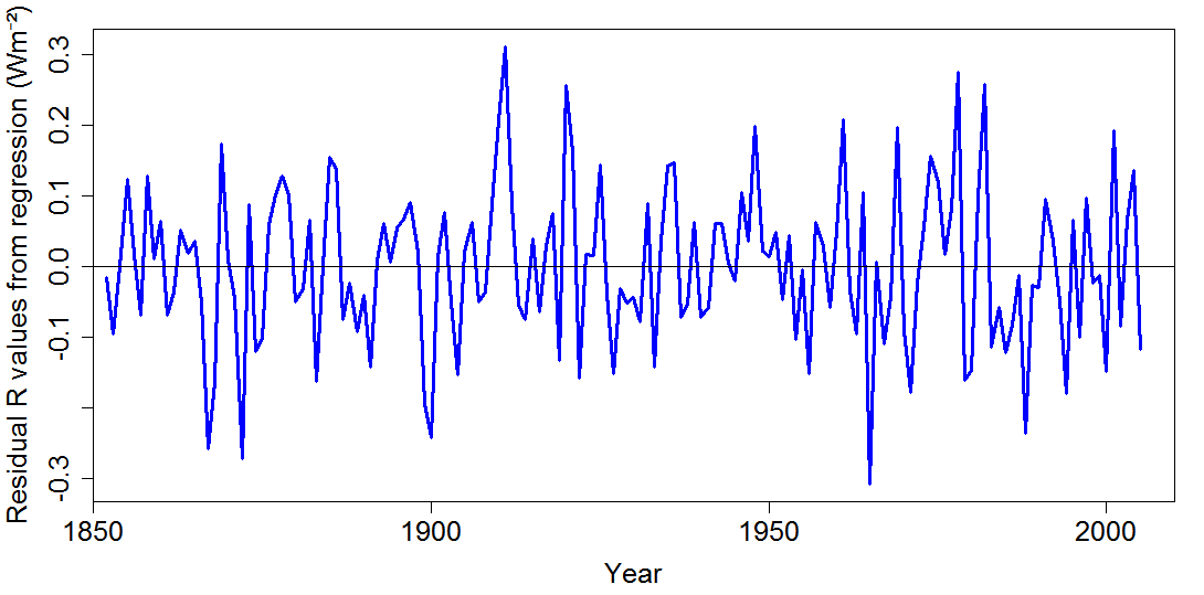
Figure 3. Residuals when regressing MPI-ESM1.1 ensemble-mean historical simulation ΔR against ΔT when land-surface warming and the low efficacy of volcanic forcing have been adjusted for.
Nor is there any evidence for the residuals being non-normal. The Shapiro-Wilk normality test gives a p-value of 0.96 (a value of ≤ 0.05 would usually be taken to reject normality). And a QQ plot of the quantiles of the residuals against those expected if their distribution were normal, with the same standard deviation as the residuals, is very close to a 1-1 line (Figure 4).
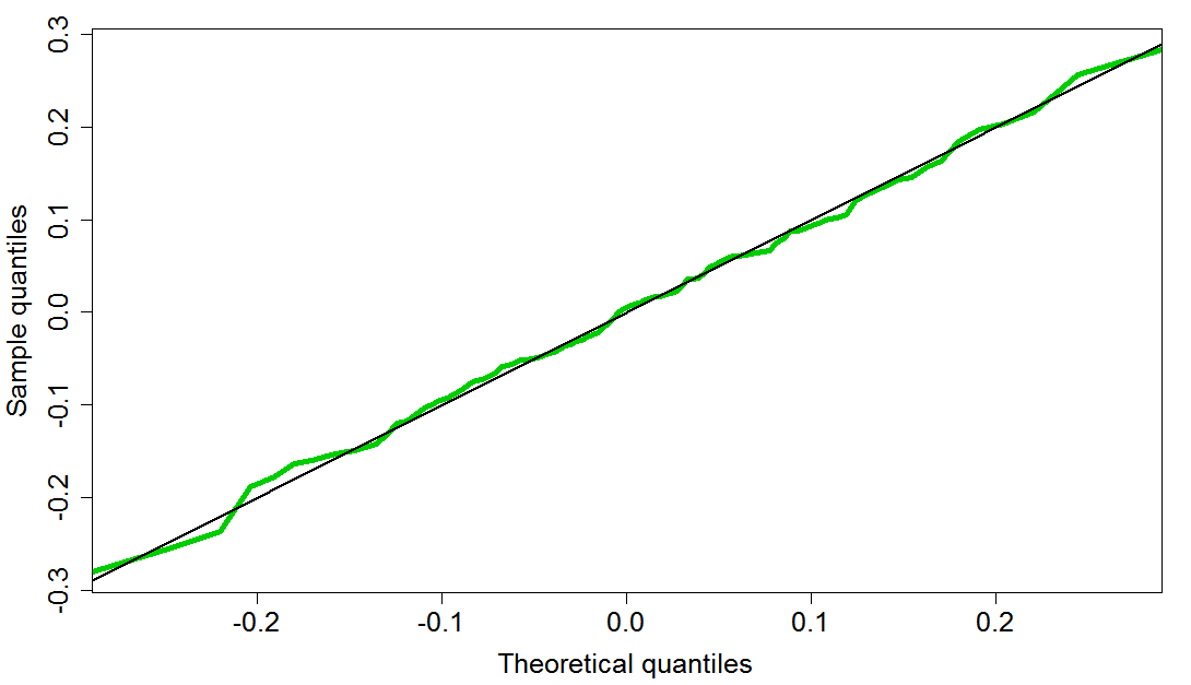
Figure 4. QQ plot for the residuals shown in Figure 1. If the residuals were exactly normally distributed the green line would coincide with the black line, given enough data points.
Moreover, the residuals in R from this regression have a standard deviation, of only 0.11 Wm−2, that is barely more than the sum in quadrature of the mean estimated standard deviations of the ensemble-mean R time series in the diagnosed ERF time series and of the ensemble-mean N time series from the 100 historical simulations, both caused by internal variability. So the contribution from any underlying variation in α must be negligible.
Results when pentadal rather than annual mean data are regressed (starting in 1851 to maximise the number of pentads) are consistent with the conclusion that the residuals are almost entirely random noise. The regression coefficients are almost identical to those for annual regression and the fit is almost perfect, with an R2 of 0.99 and a residual error standard deviation of 0.04 Wm−2. Regressing pentadal rather than annual mean data often improves noise suppression and leads to more reliable slope estimates. Gregory et al. show (their Fig.4) that when the MPI-ESM1.1 ensemble mean T is regressed against R (which is much noisier than T) rather than vice versa, the α estimate (the reciprocal of the fitted T on R regression slope) is noticeably higher. When regressing annual mean data the α estimate increases by approaching 10%, from 1.45 to 1.58 Wm−2K−1, if T is regressed on R,[12] reflecting the large regression dilution in that case. But when regressing T on R using pentadal mean data, the α estimate only increases by ~1%.
My regression results, along with the plot of the fit achieved, show that there is essentially no time-variation in α during the MPI-ESM1.1 historical simulation, provided that the low equilibrium efficacy (or, equivalently, larger climate feedback) for volcanic forcing is allowed for. It would not be possible to tell that from the solid orange line in Figure 1.
Importantly, the α of 1.45 Wm−2K−1 estimated over the historical period is very closely in line with the α of 1.43 – 1.44 Wm−2K−1 estimated from the model’s abrupt4xCO2 simulation over appropriate periods,[13] and with the α of 1.47 Wm−2K−1 estimated from the model’s 1pctCO2 simulation (in which the CO2 concentration is increased by 1% a year compound). Using that simulation provides an even closer proxy than the abrupt4xCO2 simulation for historical period CO2-only α.[14]
Although I estimated the required adjustment for volcanic forcing by regressing mean values from the 100-member ensemble, regressing instead values from individual runs also works well. The resulting α estimates have a mean (and median) of 1.46 Wm−2K−1, almost identical to α estimated from regressing ensemble-mean values. Their standard deviation is 0.08 Wm−2K−1, the same as when AR5 volcanic forcing is not included as a regressor.
I have shown that there is no evidence whatsoever that α actually varied over the course of the MPI-ESM1.1 historical simulation (provided diagnosed ERF is adjusted for land-surface warming and the low efficacy of volcanic forcing is accounted for). Accordingly, the large fluctuations of the solid orange line in Figure 1 must be regarded as due simply to the influence of low-efficacy volcanic forcing, with contributions from ERF not having been adjusted for land-surface warming and from random variability (principally in R).
Other evidence: GISS-E2-R
Although it is impossible to prove that the same is true for the CMIP5 multimodel-mean given that no accurate estimate of CMIP5 mean historical simulation ERF is available, a historical forcing time series has been diagnosed for one CMIP5 model (GISS-E2-R). Unfortunately, this is for instantaneous radiative forcing, not for ERF, so there is some uncertainty involved.[15] For the GISS-E2-R historical simulation annual ensemble-mean, a linear fit of R on T and AR5 volcanic forcing gives an R2 of 0.94 (a correlation of 0.97). The residuals are slightly larger than for the MPI-ESM1.1 ensemble-mean, as averaging is over only 6 rather than 100 runs, but they show no evidence of non-normality or significant autocorrelation. The excellent fit and satisfactory residuals strongly suggest that α was stable during the GISS-E2-R historical simulation. Moreover, the α estimate of 2.08 Wm−2K−1 is closely in line with α estimated by regression over appropriate periods of data from the model’s idealised CO2-forced simulations.[16]
Thus, for both MPI-ESM1.1 and GISS-E2-R, α estimated over the historical period is, provided an efficacy adjustment is made for volcanic forcing (e.g., by estimating it simultaneously with α), both stable and closely in line with its value as estimated from idealised CO2-only forcing simulations over periods providing a comparable forcing duration. There is therefore no evidence here for a different α value applying to aerosol forcing (as suggested by some authors)[17] [18] or to any other significant component of historical forcing apart from volcanism[19], or for any underlying variation in climate feedback strength in AOGCMs during their historical simulations.
Summary and Conclusions
Volcanic ERF has a low equilibrium efficacy, or equivalently a higher α value applies to it, relative to historical period non-volcanic ERF. This is in agreement with what Gregory et al. (2019) conclude.
Provided that the low efficacy of volcanic forcing is adjusted for:
- there is no evidence of any forced variation of α during the historical period in MPI-ESM1.1, the only model for which it is possible to determine this accurately.
- nor is there any such evidence in GISS-E2-R, the only CMIP5 model with diagnosed forcing
- in both cases estimated α is very close to α estimated from comparable CO2-only forced abrupt4xCO2 and 1pctCO2 simulation data, implying that greenhouse gas and non-volcanic non-greenhouse gas historical simulation ERF has a very similar equilibrium efficacy (or, equivalently, α is very similar for both).
While these findings go beyond those in Gregory et al. (2019), they are not inconsistent with anything in the paper.
While there is no reason to believe that the behaviour of other CMIP5 models in their historical simulations, in aggregate or individually, is different, it is impossible to confirm or disprove that because of the inability to form a good estimate of the evolution of ERF in those simulations, either in aggregate or individually.
Estimating α during the historical period by OLS regression over sliding 30-year periods, without adjusting for the low efficacy of volcanic forcing, is not the best way of examining whether and how climate feedback varied over the historical period, with any underlying variation in α being obscured by fluctuations resulting from the low efficacy of volcanic forcing and here also (to a lesser extent) from inaccurately estimated historical ERF.
Nicholas Lewis October 2019
[1] The equilibrium efficacy of a forcing agent is the ratio of α when changes are driven by an increase in CO2 forcing to α when changes are driven by an increase in forcing by that agent (Marvel et al 2016). It can be viewed as the ratio, for that agent, of the ultimate effective radiative forcing to the chosen forcing measure. For a few forcing agents, the conventional fixed-SST measure of ERF does not result in a unit equilibrium efficacy.
[2] Lewis, N. and Curry, J.A., 2015. The implications for climate sensitivity of AR5 forcing and heat uptake estimates. Climate Dynamics, 45(3-4), pp.1009-1023.
[3] Gregory, J.M., Andrews, T., Good, P., Mauritsen, T. and Forster, P.M., 2016. Small global-mean cooling due to volcanic radiative forcing. Climate Dynamics, 47(12), pp.3979-3991.
[4] I tried using regression to estimate what scaling of IPCC AR5 aerosol and volcanic and solar forcing results in the best fit of ΔR to ΔT for CMIP5-mean historical simulation data. However, the resulting residuals were dominated by spikes around volcanic episodes. It appears that the requisite scaling of AR5 volcanic forcing varies between the various eruptions, and that the time-profile of volcanic episodes may not quite match between CMIP5 and AR5. Moreover, the residuals show apparent trends over differing sub-periods, suggesting that the time-profile and not just the scaling of aerosol forcing differ between AR5 and the CMIP5-mean.
[5] Dessler AE, Mauritsen T, Stevens B (2018) The influence of internal variability on Earth’s energy balance framework and implications for estimating climate sensitivity. Atmos Chem Phys 18:5147–5155. https ://doi.org/10.5194/acp-18-5147-2018
[6] That would account for diagnosed forcing in 1850 and 1851 being lower than those for all other non-volcanic years in the 1850s despite solar forcing being high in those years.
[7] However, GISS do correct for land surface warming in their fixed-SST estimates of ERF
[8] The 7% upwards adjustment to ERF is based on the 0.052 KW−1m2 ratio of the changes in mean near-surface air temperature and in TOA radiative imbalance between 1859-82 and 1999-2008, being periods near the start and at the end of the diagnostic fixed-SST simulations that are not influenced by volcanic eruptions, multiplied by 1.35 Wm−2K−1, being α estimated by regression over years 1–150 of the MPI-ESM1.1 abrupt4xCO2 simulation. The value of α applicable to land warming in the fixed-SST, historical forcing simulations is unknown but seems unlikely to differ greatly from its thus-estimated value.
[9] All stated uncertainties are 1σ (one standard deviation) unless otherwise indicated.
[10] The ratio of the mean volcanic forcing excursions as diagnosed in MPI-ESM1.1, scaled by 1.07x, and per AR5 is ~0.85 if averaged over all six major eruptions since 1850. But for the two most recent, best observed eruptions (Pinatubo and El Chinon) the ratio is ~0.77. These values are consistent with the 0.78 ratio estimated for ECHAM6.3, the atmospheric component of MPI-ESM1.1, in Gregory et al (2019).
[11] The 1852-2005 anomalies shown are relative to means over 1852–1881.
[12] With volcanic forcing included as a separate regressor in both cases.
[13] By regression over years 2-20 and 2–50 of abrupt4xCO2, which are suitable proxies for what α would have been over the historical period if forcing had been purely from a rising CO2 concentration.
[14] Obtaining α from the ratio of mean ΔR to mean ΔT over years 60–80 of the ensemble-mean from the MPI-ESM1.1 1pctCO2 simulations (in which the CO2 concentration reaches twice its original level during year 70). The value of ΔT provides an accurate estimate of the model’s transient climate response, and by adopting an estimate of the ERF for a doubling of preindustrial CO2 concentration (F2×CO2) a value for α can also be obtained. I use an estimate of 3.95 Wm−2 for F2×CO2, which produces an α estimate of 1.47 Wm−2K−1. Averaging over years 50-90 gives the same α estimate. Estimating α instead by regression of ΔR on ΔT over years 1–100 of the 1pctCO2 simulations gives an α estimate of 1.47 Wm−2K−1, whether or not an intercept term is estimated (as the ΔR and ΔT values are anomalies relative to preindustrial control simulation means, in principle no intercept should be necessary).
[15] What was diagnosed for the GISS-E2-R historical simulation was instantaneous radiative forcing at the tropopause (IRF), not ERF. I multiplied the diagnosed time series by 0.97 to convert it to estimated ERF, that being the ratio of ERF of 4.35 Wm−2 to IRF of 4.5 Wm−2 for a doubled CO2 concentration, although it is possible this ratio is inaccurate for the composite historical forcing.
[16] Regression over years 2–50 of abrupt4xCO2 gives an α estimate of 2.09 Wm−2K−1. Estimating α instead by regressing ΔR on ΔT over years 1-100 the 1pctCO2 simulation gives a value of 2.01 Wm−2K−1; regressing instead over years 1-70 or 1-140 give virtually identical estimates. So does regressing with no intercept.
[17] Shindell, D.T., 2014: Inhomogeneous forcing and transient climate sensitivity. Nature Climate Change, 4, 274–277.
[18] Rotstayn, L. D., M. A. Collier, D. T. Shindell, and O. Boucher, 2015: Why does aerosol forcing control historical global-mean surface temperature change in CMIP5 models?, J. Clim., 28, 6608–6625, doi:10.1175/jcli-d-14-00712.1.
[19] Gregory et al’s findings point in the same direction, although they only go as far as saying “This explanation does not require EffCS for anthropogenic aerosol to differ substantially from the CO2 EffCS.”
Leave A Comment