Originally a guest post on Mar 21, 2016 – 12:37 PM at Climate Audit
Introduction
In a recent article I discussed Bayesian parameter inference in the context of radiocarbon dating. I compared Subjective Bayesian methodology based on a known probability distribution, from which one or more values were drawn at random, with an Objective Bayesian approach using a noninformative prior that produced results depending only on the data and the assumed statistical model. Here, I explain my proposals for incorporating, using an Objective Bayesian approach, evidence-based probabilistic prior information about of a fixed but unknown parameter taking continuous values. I am talking here about information pertaining to the particular parameter value involved, derived from observational evidence pertaining to that value. I am not concerned with the case where the parameter value has been drawn at random from a known actual probability distribution, that being an unusual case in most areas of physics. Even when evidence-based probabilistic prior information about a parameter being estimated does exist and is to be used, results of an experiment should be reported without as well as with that information incorporated. It is normal practice to report the results of a scientific experiment on a stand-alone basis, so that the new evidence it provides may be evaluated.
In principle the situation I am interested in may involve a vector of uncertain parameters, and multi-dimensional data, but for simplicity I will concentrate on the univariate case. Difficult inferential complications can arise where there are multiple parameters and only one or a subset of them are of interest. The best noninformative prior to use (usually Bernardo and Berger’s reference prior)[1] may then differ from Jeffreys’ prior.
Bayesian updating
Where there is an existing parameter estimate in the form of a posterior PDF, the standard Bayesian method for incorporating (conditionally) independent new observational information about the parameter is “Bayesian updating”. This involves treating the existing estimated posterior PDF for the parameter as the prior in a further application of Bayes’ theorem, and multiplying it by the data likelihood function pertaining to the new observational data. Where the parameter was drawn at random from a known probability distribution, the validity of this procedure follows from rigorous probability calculus.[2] Where it was not so drawn, Bayesian updating may nevertheless satisfy the weaker Subjective Bayesian coherency requirements. But is standard Bayesian updating justified under an Objective Bayesian framework, involving noninformative priors?
A noninformative prior varies depending on the specific relationships the data values have with the parameters and on the data-error characteristics, and thus on the form of the likelihood function. Noninformative priors for parameters therefore vary with the experiment involved; in some cases they may also vary with the data. Two studies estimating the same parameter using data from experiments involving different likelihood functions will normally give rise to different noninformative priors. On the face of it, this leads to a difficulty in using objective Bayesian methods to combine evidence in such cases. Using the appropriate, individually noninformative, prior, standard Bayesian updating would produce a different result according to the order in which Bayes’ theorem was applied to data from the two experiments. In both cases, the updated posterior PDF would be the product of the likelihood functions from each experiment, multiplied by the noninformative prior applicable to the first of the experiments to be analysed. That noninformative priors and standard Bayesian updating may conflict, producing inconsistency, is a well known problem (Kass and Wasserman, 1996).[3]
Modifying standard Bayesian updating
My proposal is to overcome this problem by applying Bayes theorem once only, to the joint likelihood function for the experiments in combination, with a single noninformative prior being computed for inference from the combined experiments. This is equivalent to the modification of Bayesian updating proposed in Lewis (2013a).[4] It involves rejecting the validity of standard Bayesian updating for objective inference about fixed but unknown continuously-valued parameters, save in special cases. Such special cases include where the new data is obtained from the same experimental setup as the original data, or where the experiments involved are different but the same form of prior in noninformative in both cases.
Since standard Bayesian updating is simply the application of Bayes’ theorem using an existing posterior PDF as the prior distribution, rejecting its validity is quite a serious step. The justification is that Bayes’ theorem applies where the prior is a random variable having an underlying, known probability distribution. An estimated PDF for a fixed parameter is not a known probability distribution for a random variable.[5] Nor, self-evidently, is a noninformative prior, which is simply a mathematical weight function. The randomness involved in inference about a fixed parameter relates to uncertainty in observational evidence pertaining to its value. By contrast, a probability distribution from which a variable is drawn at random tells one how the probability that the variable will have any particular value varies with the value, but it contains no information relating to the specific value that is realised in any particular draw.
Computing a single noninformative prior for inference from the combination of two or more experiments is relatively straightforward provided that the observational data involved in all the experiments is independent, conditional on the parameter value – a standard requirement for Bayesian updating to be valid. Given such independence, likelihood functions may be combined through multiplication, as is done both in standard Bayesian updating and my modification thereof. Moreover, Fisher information for a parameter is additive given conditional independence. In the univariate parameter case, where Jeffreys’ prior is known to be the best noninformative prior, revising the existing noninformative prior upon updating with data from a new experiment is therefore simple. Jeffreys’ prior is the square root of Fisher information (h), so one obtains the updated Jeffreys’ prior (πJ.u) by simply adding in quadrature the existing Jeffreys’ prior (πJ.e) and the Jeffreys’ prior for the new experiment (πJ.n):
πJ.u = sqrt(πJ.e2 + πJ.n2 )
where πJ. = sqrt( h.).
The usual practice of reporting a Bayesian parameter estimate, whether or not objective, in the form of a posterior PDF is insufficient to enable implementation of this revised updating method. In the univariate case, it suffices to report also the likelihood function and the (Jeffreys’) prior. Reporting just the likelihood function as well as the posterior PDF is not enough, because that only enables the prior to be recovered up to proportionality, which is insufficient here since addition of (squared) priors is involved.[6]
The proof of the pudding is in the eating, as they say, so how does probability matching using my proposed method of Bayesian updating compare with the standard method? I’ll give two examples, both taken from Lewis (2013a), my arXiv paper on the subject, each of which involve two experiments: A and B.
Numerical testing: Example 1
In the first example, the observational data for each experiment is a single measurement involving a Gaussian error distribution with known standard deviation (0.75 and 1.5 for experiments A and B respectively). In experiment A, what is measured is the unknown parameter itself. In experiment B, the cube of the parameter is measured. The calculated Jeffreys’ prior for experiment A is uniform; that for experiment B is proportional to the square of the parameter value. Probability matching is computed for a single true parameter value, set at 3; the choice of parameter value does not qualitatively affect the results.
Figure 1 shows probability matching tested by 20,000 random draws of experimental measurements. The y-axis shows the proportion of cases for which the parameter value at each posterior CDF percentage point, as shown on the x-axis, exceeds the true parameter value. The black dotted line in each panel show perfect probability matching (frequentist coverage).
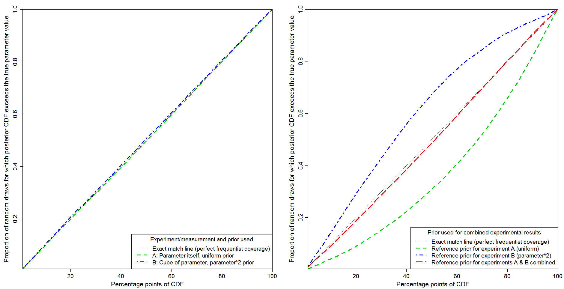 Fig 1: Probability matching for experiments measuring: A – parameter; B – cube of parameter.
The left hand panel relates to inference based on data from each separate experiment, using the correct Jeffreys’ prior (which is also the reference prior) for that experiment. Probability matching is essentially perfect in both cases. That is what one would expect, since in both cases a (transformational) location parameter model applies: the probability of the observed datum depends on the parameter only through the difference between strictly monotonic functions of the observed value and of the parameter. That difference constitutes a so-called pivot variable. In such a location parameter case, Bayesian inference is able to provide exact probability matching, provided the appropriate noninformative prior is used.
The right hand panel relates to inference based on the combined experiments, using the Jeffreys’/reference prior for experiment A (green line), that for experiment B (blue line) or that for the combined experiments (red line), computed by adding in quadrature the priors for experiments A and B, as described above.
Standard Bayesian updating corresponds to either the green or the blue lines depending on whether experiment A or experiment B is analysed first, with the resulting initial posterior PDF being multiplied by the likelihood function from the other experiment to produce the final posterior PDF. It is clear that standard Bayesian updating produces order-dependent inference, with poor probability matching whichever experiment is analysed first.
By contrast, my proposed modification of standard Bayesian updating, using the Jeffreys’/reference prior pertaining to the combined experiments, produces very good probability matching. It is not perfect in this case. Imperfection is to be expected; when there are two experiments there is no longer a location parameter situation, so Bayesian inference cannot achieve exact probability matching.[7]
Numerical testing: Example 2
The second example involves Bernoulli trials. The experiment involves repeatedly making independent random draws with two possible outcomes, “success” and “failure”, the probability of success being the same for every draw. Experiment A involves a fixed number of draws n, with the number of “failures” z being counted, giving a binomial distribution. In Experiment B draws are continued until a fixed number r of failures occur, with the number of observations y being counted, giving a negative binomial distribution.
In this example, the parameter (here the probability of failure, θ) is continuous but the data are discrete. The Jeffreys’ priors for these two experiments differ, by a factor of sqrt(θ). This means that Objective Bayesian inference from them will differ even in the case where z = r and y = n, for which the likelihood functions for experiment A and B are identical. This is unacceptable under orthodox, Subjective, Bayesian theory. That is because it violates the so-called likelihood principle:[8] inference would in this case depend on the stopping rule as well as on the likelihood function for the observed data, which is impermissible.
Figure 2 shows probability matching tested by random draws of experimental results, as in Figure 1. Black dotted lines show perfect probability matching (frequentist coverage).In order to emphasize the difference between the two Jeffreys’ priors, I’ve set n at 40, r at 2, and selected at random 100 probabilities of failure, uniformly in the range 1–11%, repeating the experiments 2000 times at each value.[9]
The left hand panel of Fig. 2 shows inference based on data from each separate experiment. Green dashed and red dashed-dotted lines are based on using the Jeffreys’ prior appropriate to the experiment involved, being respectively binomial and negative binomial cases. Blue and magenta short-dashed lines are for the same experiments but with the priors swapped. When the correct Jeffreys’ prior is used, probability matching is very good: minor fluctuations in the binomial case arise from the discrete nature of the data. When the priors are swapped, matching is poor.
The right hand panel of Fig. 2 shows inference derived from the experiments in combination. The product of their likelihood functions is multiplied by each of three candidate priors. It is multiplied alternatively by the Jeffreys’ prior for experiment A, corresponding to standard Bayesian updating of the experiment A results (green dashed line); by the Jeffreys’ prior for experiment B, corresponding to standard Bayesian updating of the experiment A results (dash-dotted blue line); or by the Jeffreys’ prior for the combined experiments, corresponding to my modified form of updating (red short-dashed line). As in Example 1, use of the combined experiments Jeffreys’ prior provides very good, but not perfect, probability matching, whilst standard Bayesian updating, of the posterior PDF from either experiment generated using the prior that is noninformative for it, produces considerably less accurate probability matching.
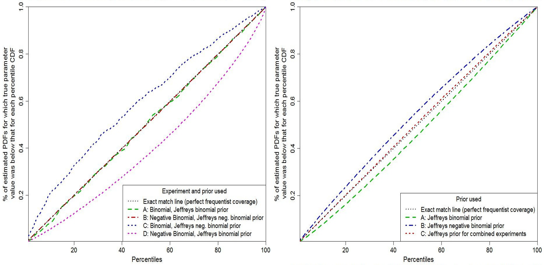 Fig 2: Probability matching for Bernoulli experiments: A – binomial; B – negative binomial.
Conclusions
I have shown that, in general, standard Bayesian updating is not a valid procedure in an objective Bayesian framework, where inference concerns a fixed but unknown parameter and probability matching is considered important (which it normally is). The problem is not with Bayes’ theorem itself, but with its applicability in this situation. The solution that I propose is simple, provided that the necessary likelihood and Jeffreys’ prior/ Fisher information are available in respect of the existing parameter estimate as well as for the new experiment, and that the independence requirement is satisfied. Lack of (conditional) independence between the different data can of course be a problem; prewhitening may offer a solution in some cases (see, e.g., Lewis, 2013b).[10]
I have presented my argument about the unsuitability of standard Bayesian updating for objective inference about continuously valued fixed parameters in the context of all the information coming from observational data, with knowledge of the data uncertainty characteristics. But the same point applies to using Bayes’ theorem with any informative prior, whatever the nature of the information that it represents.
One obvious climate science application of the techniques for combining probabilistic estimates of a parameter set out in this article is the estimation of equilibrium climate sensitivity (ECS). Instrumental data from the industrial period and paleoclimate proxy data should be fairly independent, although there may be some commonality in estimating, for example, radiative forcings. Paleoclimate data, although generally more uncertain, is relatively more informative than industrial period data about high ECS values. The different PDF shapes of the two types of estimate implies that different noninformative priors apply, so using my proposed approach to combining evidence, rather than using standard Bayesian updating, is appropriate if objective Bayesian inference is intended. I have done quite a bit of work on this issue and I am hoping to get a paper published that deals with combining instrumental and paleoclimate ECS estimates.
Nicholas Lewis
Notes and references
[1] See, e.g., Chapter 5.4 of J M Bernardo and A F M Smith, 1994, Bayesian Theory. Wiley. An updated version of Ch. 5.4 is contained in section 3 of Bayesian Reference Analysis, available at http://www.uv.es/~bernardo/Monograph.pdf
[2] Kolmogorov, A N, 1933, Foundations of the Theory of Probability. Second English edition, Chelsea Publishing Company, 1956, 84 pp.
[3] Kass, R. E. and L. Wasserman, 1996: The Selection of Prior Distributions by Formal Rules. J. Amer. Stat. Ass., 91, 435, 1343-1370. Note that no such conflict normally arise where the parameter takes on only discrete values, since then a uniform prior (equal weighting all parameter values) is noninformative in all cases.
[4] Lewis, N, 2013a: Modification of Bayesian Updating where Continuous Parameters have Differing Relationships with New and Existing Data. arXiv:1308.2791 [stat.ME] http://arxiv.org/ftp/arxiv/papers/1308/1308.2791.pdf.
[5] Barnard, GA, 1994: Pivotal inference illustrated on the Darwin Maize Data. In Aspects of Uncertainty, Freeman, PR and AFM Smith (eds), Wiley, 392pp
[6] In the multiple parameter case, it is necessary to report the Fisher information (a matrix in this case) for the parameter vector, since it is that which gets additively updated, as well as the joint likelihood function for all parameters. Where all parameters involved are of interest, Jeffreys’ prior – here the square root of the determinant of the Fisher information matrix – is normally still the appropriate noninformative prior (it is the reference prior). Where interest lies in only one or a subset of the parameters, the reference prior may differ from Jeffreys’ prior, in which case the reference prior is to be preferred. But even where the best noninformative prior is not Jeffreys’ prior, the starting point for computing it is usually the Fisher information matrix.
[7] This is related to a fundamental difference between frequentist and Bayesian methodology: frequentist methodology involves integrating over the sample space; Bayesian methodology involves integrating over the parameter space.
[8] Berger, J. O. and R. L. Wolpert, 1984: The Likelihood Principle (2nd Ed.). Lecture Notes Monograph, Vol 6, Institute of Mathematical Statistics, 206pp
[9] Using many different probabilities of failure helps iron out steps resulting from the discrete nature of the data.
[10] Lewis, N, 2013b: An objective Bayesian, improved approach for applying optimal fingerprint techniques to estimate climate sensitivity. Jnl Climate, 26, 7414–7429.
Leave A Comment