Originally posted on Jul 30, 2014 – 10:41 AM at Climate Audit
In July 2004 the IPCC held a Working Group 1 (WG1) Workshop on climate sensitivity, as part of the work plan leading up to AR4. In one session, Myles Allen of Oxford university and a researcher in his group, David Frame, jointly gave a presentation entitled “Observational constraints and prior assumptions on climate sensitivity”. They developed the work presented into what became an influential paper, Frame et al 2005,[1] here, with Frame as lead author and Allen as senior author.
Frame and Allen pointed out that climate sensitivity studies could be – whether or not they explicitly were – couched in a Bayesian formulation. That formulation applies Bayes’ theorem to produce a posterior probability density function (PDF), from which best estimates and uncertainty ranges are derived. The posterior PDF represents, at each value for climate sensitivity (ECS), and of any other parameters (fixed but uncertain variables) being estimated, the product of the likelihood of the observations at that value and the “prior” for the uncertain parameters that is also required in Bayes’ theorem.
Obviously, the posterior PDF, and hence the best estimate and upper uncertainty bound for ECS, depend on the form of the prior. Both the likelihood and the prior are defined over the full range of ECS under consideration. The prior can be viewed as a weighting function that is applied to the likelihood (and can be implemented by a weighted sampling of the likelihood function), but in terms of Bayes’ theorem it is normally viewed as constituting a PDF for the parameters being estimated prior to gaining knowledge from the data-based likelihood.
Frame et al 2005 stated that, unless warned otherwise, users would expect an answer to the question “what does this study tell me about X, given no knowledge of X before the study was performed”. That is certainly what one would normally expect from a scientific study – the results should reflect, objectively, the data used and the outcome of the experiment performed. In Bayesian terms, it implies taking an “Objective Bayesian” approach using a “noninformative” prior that is not intended to reflect any existing knowledge about X, rather than a “Subjective Bayesian” approach – which involves the opposite and produces purely personal probabilities.
Frame and Allen claimed that the correct prior for ECS – to answer the question they posed – depended on why one was interested in knowing ECS, and that the prior used should be uniform (flat) in the quantity in which one was interested. Such a proposal does not appear to be supported by probability theory, nor to have been adopted elsewhere in the physical sciences. Although for some purposes they seem to have preferred a prior that was uniform in TCR, their proposal implies use of a uniform in ECS prior when ECS is the target of the estimate. AR4 pointed this out, and adopted the Frame et al 2005 proposal of using a uniform in ECS prior when estimating ECS. Use of a uniform prior for ECS resulted in most of the observational ECS estimates given in Figure 9.20 and Table 9.3 of AR4 having very high 95% uncertainty bounds.
Consistent with the foregoing thesis, Frame et al 2005 stated that “if the focus is on equilibrium warming, then we cannot rule out high sensitivity, high heat uptake cases that are consistent with, but nonlinearly related to, 20th century observations”. Frame and Allen illustrated this in their 2004 presentation with ECS estimates derived from a simple global energy balance climate model, with forcing from greenhouse gases only. The model had two adjustable parameters, ECS and Kv – here meaning the square root of effective ocean vertical diffusivity. The ‘observable’ variables – the data used, errors in which are assumed to be independent – were 20th century warming attributable to greenhouse gases (AW), as estimated previously using a pattern-based detection and attribution analysis, and effective heat capacity (EHC) – the ratio of the changes in ocean heat content and in surface temperature over a multidecadal period.
Frame and Allen’s original graph (Figure 1) showed that use of a uniform prior in ECS gives a very high 95% upper bound for climate sensitivity, whereas a uniform prior in Feedback strength (the reciprocal of ECS) – which declines with ECS squared – gives a low 95% bound. A uniform prior in the observable variables (AW and EHC) also gives a 95% bound under half that based on a uniform in ECS prior; using a prior that is uniform in transient climate response (TCR) rather than in AW, and is uniform in EHC, gives an almost identical PDF.
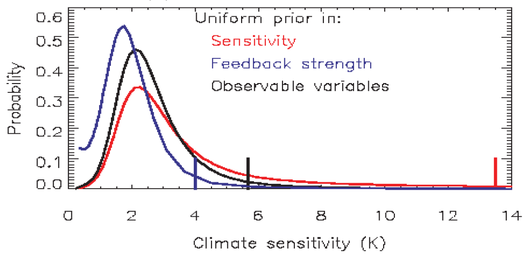 Figure 1: reproduction of Fig. (c) from Frame and Allen ‘Observational Constraints and Prior Assumptions on Climate Sensitivity’, 2004 IPCC Workshop on Climate Sensitivity. Vertical bars show 95% bounds.
However, the Frame et al 2005 claim that high sensitivity, high heat uptake cases cannot be ruled out is incorrect: such cases would give rise to excessive ocean warming relative to the observational uncertainty range. It follows that Frame and Allen’s proposal to use a uniform in ECS prior when it is ECS that is being estimated does not in fact answer the question they posed, as to what the study tells one about ECS given no prior knowledge about it. Of course, I am not the first person to point out that Frame and Allen’s proposal to use a uniform-in-ECS prior when estimating ECS makes no sense. James Annan and Julia Hargreaves did so years ago.
Frame et al 2005 was a short paper, and it is unlikely that many people fully understood what the authors had done. However, once Myles Allen helpfully provided me with data and draft code relating to the paper, I discovered that the analysis performed hadn’t actually used likelihood functions for AW and EHC. The authors had mistakenly instead used (posterior) PDFs that they had derived for AW and EHC, which are differently shaped. Therefore, the paper’s results did not represent use of the stated priors. And although, I am told, the Frame et al 2005 authors had no intention of using an Objective Bayesian approach, the PDFs they derived for AW and EHC do appear to correspond to such an approach.
Now, it is simple to form a joint PDF for AW and EHC by multiplying their PDFs together. Having done so, the model simulation runs can be used to perform a one-to-one translation from AW–EHC to ECS–Kv coordinates, and thereby to convert the PDF for AW–EHC into a PDF for ECS–Kv using the standard transformation-of-variables formula. That formula involves multiplication by the ‘Jacobian’ [determinant], which converts areas/volumes from one coordinate system to another. The standard Bayesian procedure of integrating out an unwanted variable, here Kv, then provides a PDF for ECS. The beauty of this approach is that conversion of a PDF upon a transformation of variables gives a unique, unarguably correct, result.
What this means is that, since Frame and Allen had started their ‘Bayesian’ analysis with PDFs not likelihood functions, there was no room for any argument about choice of priors; priors had already been chosen (explicitly or implicitly) and used. Given the starting point of independent estimated PDFs for AW and EHC, there was only one correct joint PDF for ECS and Kv, and there was no dispute about obtaining a marginal PDF for ECS by integrating out Kv. The resulting PDF is what the misnamed black ‘Uniform prior in Observable variables’ curve in Figure 1 really represented.
Even when, unlike in Frame and Allen’s case, the starting point is likelihood functions for the observable variables, there are attractions in applying Bayes’ theorem to the observable (data) variables (in some cases after transforming them), at which point it is often obvious which prior is noninformative, thereby obtaining an objective joint PDF for the data variables. A transformation of variables can then be undertaken to obtain an objective joint posterior PDF for the parameters. I used this approach in a more complicated situation in a 2013 climate sensitivity study,[2] but it is not in common use.
After I discovered the fundamental errors made by the Frame et al 2005 authors, I replicated and extended their work, including estimating likelihood functions for AW and EHC, and wrote a paper reanalysing their work. As well as pointing out the errors in Frame et al 2005 and, more importantly, its misunderstandings about Bayesian inference, the case provided an excellent case-study for applying the transformation of variables approach, and for comparing estimates for ECS using:
- a Bayesian method with a uniform in ECS (and Kv) prior, as Frame and Allen advocated;
- an Objective Bayesian method with a noninformative prior;
- a transformation of variables from the joint PDF for (AW, EHC); and
- a non-Bayesian profile likelihood method.
All except method 3. estimate ECS directly from likelihood functions for AW and EHC. Since those two likelihood functions were not directly available, I estimated each of them from the related PDF. I did so by fitting to each of those PDFs a parameterised probability distribution for which I knew the corresponding noninformative prior, and then dividing it by that prior. This procedure effectively applies Bayes’ theorem in reverse, and seems to work well provided the parameterised probability distribution family chosen offers a close match to the PDF being fitted.
The profile likelihood method– an objective non-Bayesian method not involving any selection of a prior – provides approximate confidence intervals. Such intervals are intended to reflect long-run frequencies on repeated testing, and are conceptually different from Bayesian probability estimates. However, noninformative priors for Objective Bayesian inference are often designed so that the resulting posterior PDFs provide uncertainty ranges that closely replicate confidence intervals.
The ECS estimates resulting from the various methods are shown in Figure 2, a slightly simplified version of Figure 5 in my paper.
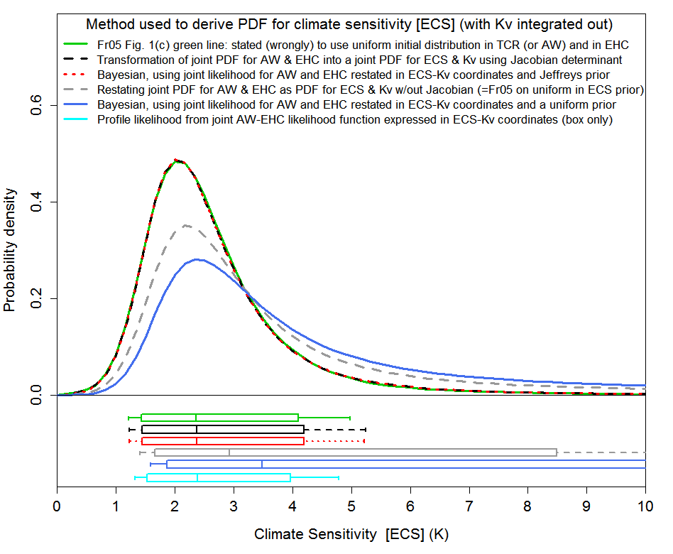 Figure 2. Estimated marginal PDFs for climate sensitivity (in K or °C) derived on various bases. The box plots indicate boundaries, to the nearest grid value, for the percentiles 5–95 (vertical bar at ends), 10-90 (box-ends), and 50 (vertical bar in box: median), and allow for off-graph probability lying between ECS = 10°C and ECS = 20°C. (The cyan box plot shows confidence intervals, the vertical bar in the box showing the likelihood profile peak).
Methods 2 and 3 [the red and black lines and box plots in Figure 2] give identical results – they logically must do in this case. The green line, from Frame et al 2005, is an updated version of the black line in Figure 1, using a newer ocean heat content dataset. The green line’s near identity to the black line confirms that it actually represents a transformation of variables approach using the Jacobian. Method 4 [the cyan box plot in Figure 2], profile likelihood, gives very similar results. That similarity strongly supports my assertion that methods 2 and 3 provide objectively-correct ECS estimation, given the data and climate model used and the assumptions made. Method 1, use of a uniform prior in ECS (and in Kv), [blue line in Figure 2] raises the median ECS estimate by almost 50% and overestimates the 95% uncertainty bound for ECS by a factor of nearly three. The dashed grey line shows the result of Frame et al 2005’s method of estimating ECS that claimed to use a uniform prior in ECS and Kv, but which in fact equated to using the transformation of variables method without including the required Jacobian factor.
For the data used in Frame et al 2005, the objective estimation methods all give a best (median) estimate for ECS of 2.4°C. Correcting for an error in Frame et al 2005’s calculation of the ocean heat content change reduces the best estimate for ECS to 2.2°C, still somewhat higher than other estimates I have obtained. That is very likely because Frame et al 2005 used an estimate of attributable warming based on 20th century data, which has been shown to produce excessive sensitivity estimates.[3]
The noninformative prior used for method 2 is shown in Figure 3. The prior is very highly peaked the in low ECS, low Kv corner, and by an ECS of 5°C is, at mid-range Kv, under one-hundredth of its peak value . What climate scientist using a Subjective Bayesian approach would choose a joint prior for ECS and Kv looking like that, or even include any prior like it if exploring sensitivity to choice of priors? Most climate scientists would claim I had chosen a ridiculous prior that ruled out a priori the possibility of ECS being high. Yet, as I show in my paper, use of this prior produces identical results to those from applying the transformation of variables formula to the PDFs for AW and EHC that were derived in Frame et al 2005, and almost the same results as using the non-Bayesian profile likelihood method.
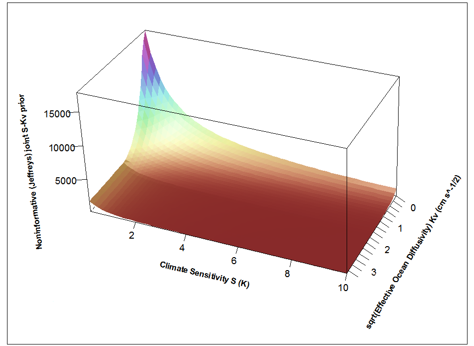
Figure 3: Noninformative Jeffreys’ prior for inferring ECS and Kv from the (AW, EHC) likelihood. (The fitted EHC distribution is parameterised differently here than in my paper, but the shape of the prior is almost identical.)
Use of a uniform prior for ECS in Bayesian climate sensitivity studies has remained common after AR4, with the main alternative being an ‘expert prior’ – which tends to perpetuate the existing consensus range for ECS. The mistake many scientists using Bayesian methods make is thinking that the shape of a prior simply represents existing probabilistic knowledge about the value of the parameter(s) concerned. However, the shape of a noninformative prior – one that has minimal influence, relative to the data, on parameter estimation – represents different factors. In particular, it reflects how the informativeness of the data about the parameters varies with parameter values, as the sensitivity of the data values to parameter changes alters and data precision varies. Such a prior is appropriate for use when either there is no existing knowledge or – as Frame et al 2005 correctly imply is normal in science – parameter estimates are to be based purely on evidence from the study, disregarding any previous knowledge. Even when there is existing probabilistic knowledge about parameters and that knowledge is to be incorporated, the prior needs to reflect the same factors as a noninformative prior would in addition to reflecting that knowledge. Simply using an existing estimated posterior PDF for the parameters as the prior distribution will not in general produce parameter estimates that correctly combine the existing knowledge and new information.[4]
Whilst my paper was under review, the Frame et al 2005 authors arranged a corrigendum to Frame et al 2005 in GRL in relation to the likelihood function error and the miscalculation of the ocean heat content change. They did not take the opportunity to withdraw what they had originally written about choice of priors, or their claim about not being able to rule out high ECS values based on 20th century observations. My paper[5] is now available in Early Online Release form, here. The final submitted manuscript is available on my own webpage, here.
Nicholas Lewis
[1] Frame DJ, BBB Booth, JA Kettleborough, DA Stainforth, JM Gregory, M Collins and MR Allen, 2005. Constraining climate forecasts: The role of prior assumptions. Geophys. Res. Lett., 32, L09702
[2] Lewis, N., 2013. An objective Bayesian improved approach for applying optimal fingerprint techniques to estimate climate sensitivity. Journal of Climate, 26, 7414-7429.
[3] Gillett et al, 2012. Improved constraints on 21st-century warming derived using 160 years of temperature observations. Geophys. Res. Lett., 39, L01704
[4] Lewis, N., 2013. Modification of Bayesian Updating where Continuous Parameters have Differing Relationships with New and Existing Data. arXiv:1308.2791 [stat.ME].
[5] Lewis N, 2014. Objective Inference for Climate Parameters: Bayesian, Transformation of Variables and Profile Likelihood Approaches. Journal of Climate, doi:10.1175/JCLI-D-13-00584.1
Postscript
James Annan had a blog post about his and Julia Hargreaves’ efforts to get their criticisms of the use of a uniform prior for ECS estimation published, here. Their paper, “On the generation and interpretation of probabilistic estimates of climate sensitivity”, Climatic Change, 2011, 104, 3-4, pp 423-436, is available here.
Leave A Comment