A pdf copy of this article is available here
This is a brief comment on a new paper[i] by a mathematician in the Exeter Climate Systems group, Femke Nijsse, and two better known colleagues, Peter Cox and Mark Williamson. I note that Earth Systems Dynamics published the paper despite one of the two peer reviewers recommending against acceptance without further major revisions. But neither of the reviewers appear to have raised the issue that I focus on here.
“Emergent constraints” methods relate observable climate trends, variations or other variables to climate system properties of interest, such as equilibrium climate sensitivity (ECS), in an ensemble of models. They then use the observed values of the variable(s) involved to estimate ECS or the other properties of interest. I’m not a great fan of emergent constraints studies, the results of which are often sensitive to the model ensemble used. Here the emergent constraint is the relationship, assumed linear, between transient climate response (TCR) and global warming from 1975 onwards.
The authors thereby derive, from a CMIP6 26 model ensemble, a TCR estimate of 1.68 K (16-84% ‘likely’ range 1.29–2.05 K, 5-95% range 1.0–2.3 K) using warming up to 2019.
The paper states that using instead warming up to 2014, thereby enabling use of a larger set of CMIP6 models, reduces the TCR estimate to 1.54 K (5-95% range 0.76–2.30 K), but don’t mention that in their abstract or conclusions.
The authors also derive an estimated likely range for ECS of 1.9–3.4 K (5–95% range 1.5–4.0 K) from CMIP6 models, median estimate 2.6 K, from warming to 2019. Based on warming up to 2014 in the larger ensemble of CMIP6 models, the median ECS estimate is 1.9 K (5–95% range 1.0–3.3 K). Again, the result from the larger ensemble is not mentioned in the abstract or conclusions.
I am very doubtful about estimating ECS by comparing observed and simulated historical warming. Without also using observational data on ocean heat update, to estimate changes in the Earth’s energy imbalance, it is impossible to distinguish satisfactorily between ECS and ocean heat uptake both being high and them both being low – either combination can produce the same historical warming. So I would not place any reliance on their ECS ranges, even if they don’t look unreasonable.
On the other hand, one would expect historical warming in climate models to have a close to linear relationship with their TCR, since pre-1975 ‘warming in the pipeline’ is fairly negligible and post 1975 forcing is reasonably close to the quasi-linear ramp forcing used to measure TCR, and similarly of multidecadal length. The existence of episodic volcanic forcing, to which models and the real climate system may respond differently, is a possible confounding factor, although use of the difference between 1975–1985 and the 2009–2019 means to measure warming excludes years affected by the 1991 Mount Pinatubo eruption. There is also the issue that the mean change in effective radiative forcing (ERF) in climate models between those two periods may not equal the ERF change in the real climate system. For CMIP5 models at least, I suspect that their mean ERF change falls somewhat short of the actual change. That would induce an upwards bias in the emergent constraint TCR estimate.
Regardless of the above considerations, there is a fatal problem with the regression method used to relate TCR with warming. If a model has a TCR of zero, then it would be expected to show zero historical warming. The authors appear to recognise this, writing “As no warming would be expected if climate sensitivity were zero, we expect the regression to pass through the intercept”. They actually mean pass through the origin (have a zero y-intercept), as their equations (A3) and (A4) make clear. And their equation (3) theoretical relationship between TCR and warming, TCR = s ΔT, has no offset term. It is therefore physically inappropriate to use regression with a y-intercept term being estimated.
However, despite admitting that a zero y-intercept is physically appropriate, the study estimates a regression fit using a y-intercept as well as a slope coefficient parameter. Moreover, the resulting best-fit line does not pass at all close to the origin. Their estimate implies that climate models with a TCR of ~0.7 K would have simulated zero post-1975 warming. Their Figure 4(a), reproduced as Figure 1 below, shows this.
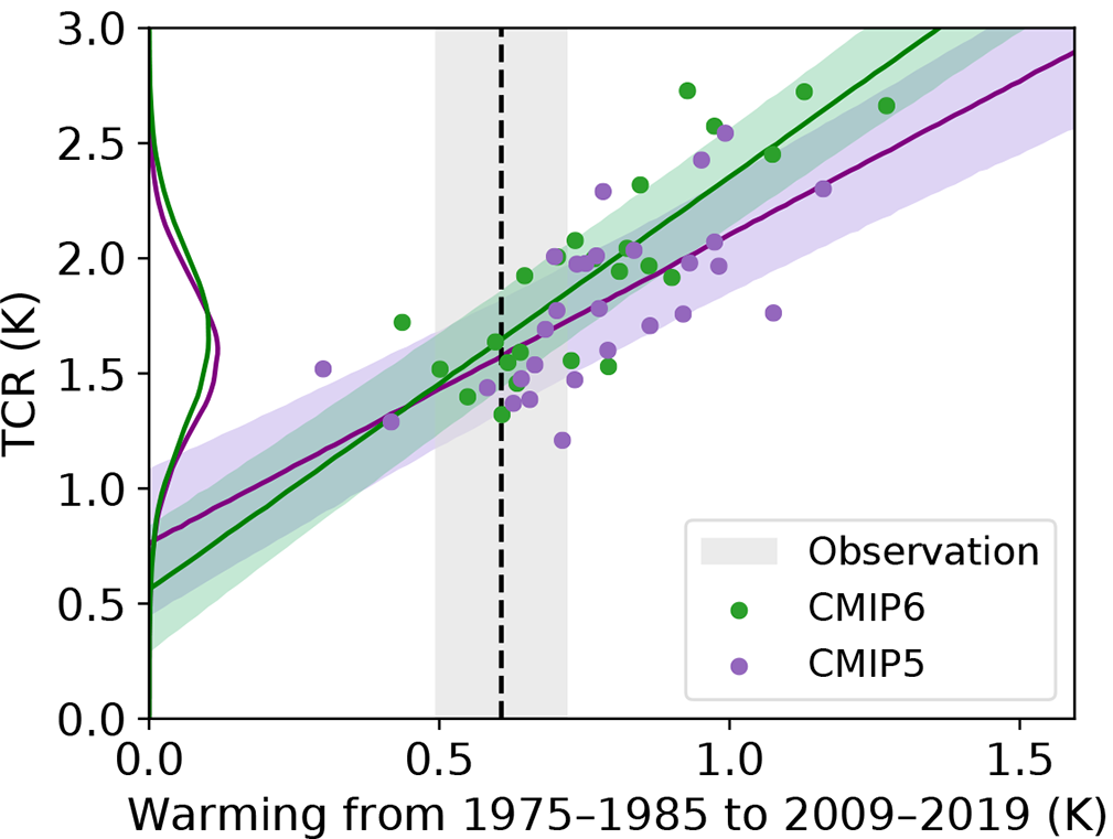
Figure 1. Reproduction of Figure 4(a) of Nijsse et al. (2020). Emergent constraint on TCR against historical warming ΔT. ΔT is calculated from the difference between 1975–1985 and 2009–2019 of a time series of GMSAT. Linear regression is performed with all CMIP5 and CMIP6 simulations. Shaded areas indicate a 90% prediction interval. The vertical dashed line is the mean value of the observations, and the y axis shows the probability distribution of both generations of ensembles.
A quite involved and not very clearly described hierarchical Bayesian model regression method is used, which makes it difficult to reproduce exactly the study’s results. Remarkably, the numerical value and uncertainty range of the observed warming estimate is nowhere stated. I therefore measured it off their Figure 4(a), as 0.606 K, and took the shading as showing a normally distribution 5–95% range, width 0.225 K. Based on a simple ordinary least squares (OLS) with-intercept regression of TCR on model-ensemble mean simulated historical warming, across the multimodel combined CMIP5 and CMIP6 ensemble, I estimate a median TCR estimate of 1.62 K (or 1.66 K using the CMIP6 ensemble alone – marginally lower than their 1.68 K).
If I repeat the exercise but without estimating a y-intercept, thereby forcing the regression fit to match a zero TCR with zero historical warming, the emergent constraint gives a TCR best estimate of 1.43 K. The regression fit is very good (R2 = 0.97). There is little regression dilution when no y-intercept is estimated. Regressing warming on TCR rather than vice versa gives an emergent constraint TCR best estimate of 1.47 K. Regressing TCR on warming just across the CMIP5 ensemble gives a slightly lower TCR estimate of 1.37 K (R2 = 0.97). Doing so across the CMIP6 ensemble alone gives a TCR estimate of 1.50 K ((R2 = 0.98). The slope coefficient standard errors imply that there is only a 3.1% chance that the TCR–warming relationship is the same in the CMIP5 and CMIP6 ensembles.
It is unclear which regression method is more accurate. Using the geometrical mean of the estimates regressing each way, as is sometimes recommended, gives a TCR best estimate of 1.45 K from the combined CMIP5/CMIP6 ensemble. A crude estimate of uncertainty can be obtained by using, for each type of regression, the standard error in the slope estimate and the observational uncertainty to form a large number of randomly sampled TCR estimates, combining the two resulting sets of estimates and computing quantiles. Doing so gives a median TCR estimate of 1.45 K, with a 16–84% range of 1.29–1.62 K and a 5–95% range of 1.18–1.74 K. However, this does not account for all sources of uncertainty.
Interestingly, when fitting a relationship between ECS and post-1975 warming, and between ECS and TCR, the authors didn’t use a y-intercept term, resulting in those fits passing through the origin.
My key point is that an analysis method that results in a physically reasonable estimated relationship between the variables being studied should be used. An estimated relationship that implies zero warming with a positive TCR, and significant cooling with a zero TCR, is unphysical. Therefore, the results of the Nijsse et al. paper are unreliable and should be discounted.
Nicholas Lewis 19 August 2020 (minor corrections, mainly to the third paragraph, made 20 August 2020)
[i] Njisse et al., 2020: Emergent constraints on transient climate response (TCR) and equilibrium climate sensitivity (ECS) from historical warming in CMIP5 and CMIP6 models, Earth Syst. Dynam., 11, 737–750, 2020 https://doi.org/10.5194/esd-11-737-2020
Leave A Comment